Matrix form of Linear Regression The F distribution

Matrix form of Linear Regression The F distribution ANOVA approach to Linear Regression ANOVA approach to t-test (One way ANOVA with two levels)

X <- c(30, 20, 60, 80, 40, 50, 60, 30, 70, 60) Y <- c(73, 50, 128, 170, 87, 108, 135, 69, 148, 132) Y = B 0 + B 1 X + e = B 0 + B 1 + Linear least square fit finds B 0 and B 1 to guarantee that is a minimum

By setting “x=true”, we can keep R’s version of the matrices used to find the parameters

We can get R to give us all of the pieces used in the fit… Y = B 0 + B 1 X + e

We can make this even more concise… Hastie et al: The elements of Statistical Learning http: //www-stat. stanford. edu/~tibs/Elem. Stat. Learn/download. html

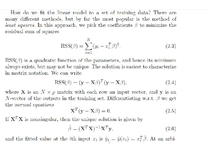
So we can find least square parameters easily with a few line of matrix manipulation

Matrix form of Linear Regression The F distribution ANOVA approach to Linear Regression ANOVA approach to t-test (One way ANOVA with two levels)

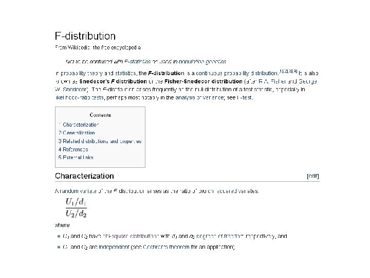
The F distribution is built on the Chi-square distribution… Neter et al - Applied Linear Statistical Models

As usual df, pf, qf, rf….

You can guess how to use these methods without looking at the documentation… Here is a demonstration that the definition of F is correct…

Matrix form of Linear Regression The F distribution ANOVA approach to Linear Regression ANOVA approach to t-test (One way ANOVA with two levels)

We have Y = B 0 + B 1 X + e We want to know if B 1 is significantly different than 0. In the previous lecture, we saw how to do this with the t-distribution. That’s what R gives us when we type summary()

Alternatively, we can compare the error of the full model: Y = B 0 + B 1 X + e 8 d. f. associated with this model (there are 2 parameters with 10 data points) How much error would we have if B 1 is equal to 0 in the reduced model? Y = B 0 + e The value of B 0 that minimizes the error is just the mean. So the sum squared error is There are 9 d. f. associated with this model (there is 1 parameter with n=10)

Our ANOVA statistic is: (reduced error – full error)/ (reduced DF – full DF) (Full error)/ (full DF) ( 13660 – 60 ) / (9 -8 ) (60)/ (8) (13600) / 1 = = 1813. 3 7. 5 If the parameter didn’t make much of a difference, the full and reduced error would be similar…. In this case, the extra parameter makes a huge difference We say, this is F distributed with df = (1, 8) This is what R does when we type ANOVA (lm) Zeros out the parameters and asks whether the error changes by a significant amount

Visually Neter et al - Applied Linear Statistical Models

We can define R 2 as: Regression sum squared (SSR) = R 2 measures how much variance your model captures Total sum squared ( SSTO )

R is the Pearson Correlation co-efficient (which is likely familiar to all of you!) R 2 R R 2 > r <- sum(( X- mean(X)) * (Y - mean(Y))) / ( sqrt(sum((X-mean(X)) * (X-mean(X)) )) * sqrt(sum((Y-mean(Y)) * (Y-mean(Y)) ))) >r*r [1] 0. 9956076 http: //en. wikipedia. org/wiki/Pearson_product-moment_correlation_coefficient

Note that if we scramble the Y data, the significance of the relationship is lost The residuals for the reduced model haven’t changed: However, the full model now doesn’t explain very much (reduced-full) / full = ((13660 -13400. 12) / 1 ) / (13400. 12/8) = F-statistic = 0. 1552;

In summary, R fits the linear model and gives us a great deal of information on the fit T derived errors on B 0 and B 1 Stats on the residuals B 0 B 1 R 2 P-value from F test ANOVA F statistic Sqrt( sum( residuals)) / model df = sqrt( 60 / 8 ) =

ANOVA() tells R to zero out each (non-intercept) parameter and evaluate significance that way Divided by D. F. (in this case 1 since there is one parameter different between reduced and full) P-value from F-test Divided by D. F. (in this case 8 since we estimate two parameters from 10 data points)

Matrix form of Linear Regression The F distribution ANOVA approach to Linear Regression ANOVA approach to t-test (One way ANOVA with two levels)

Previously: We saw the two sample t-test. So consider two samples (weight of mice on Drug A vs. Drug B) Consider the equal variance version of the t-test rm(list=ls()) a <- c(2. 1, 3. 2, 2. 0, 1. 9) b <- c(1. 8, 1. 3, 1. 7, 1. 2, 1. 1) t. test(a, b, var. equal=TRUE) (In the ANOVA version of the t-test, the samples must have equal variance!)

We can make an alternative version of this test cast as an ANOVA rm(list=ls()) a <- c(2. 1, 3. 2, 2. 0, 1. 9) b <- c(1. 8, 1. 3, 1. 7, 1. 2, 1. 1) ( my. Data <- c(a, b) ) ( categories <- c( rep('A', length(a)), rep('B', length(b)) ) ) ( categories <- factor(categories) ) my. Lm <- lm( my. Data ~ categories, x=TRUE) anova(my. Lm) We tell R that we have a categorical variable This is a ONE-way ANOVA (with 2 levels) One factor (two levels)

The full model has sum squared residual of 1. 488 with 7 d. f. = B 0 + B 1 +

The reduced model (B 1=0) has sum squared residual 3. 208889 with 8 d. f. = B 0 + The errors will be minimized when B 0 = mean of data

Our ANOVA statistic is f=: (reduced error – full error)/ (reduced DF – full DF) (Full error)/ (full DF) ( ( 3. 208889 - 1. 488 ) / 1 ) / (1. 488 /7 ) So t. test, anova and summary all yield identical results. .

“Full model” ; 7 degrees of freedom (n=9 – 2 parameters). The mean of A and B are modeled as distinct The mean of A The difference between the mean of A and the mean of B. A is the “background” ; B is compared to A. We can switch that with relevel The null hypothesis is that this is zero (i. e. that mean(A) == mean(B))

“Reduced model” ; 8 degrees of freedom (n=9 – 1 parameters). There is only one grand mean. The ANOVA asks does the full model explain significantly more of the data than does the reduced model? The null hypothesis is that the data is explained best by one mean

In the previous slide, A is the “background” ; B is compared to A. We can switch that with relevel ; now “B” is the background The mean of A The mean of B The difference between the mean of B and the mean of A. The null hypothesis is that this is zero (i. e. that mean(A) == mean(B)) For the 2 level ANOVA it doesn’t matter which is “background”; we get the same p-value

With “A” as the background…. = B 0 + B 1 + With “B” as the background…. = B 0 + B 1 + For the 2 level case, these models produce identical inference (it doesn’t matter which is background); This gets more complicated as we move to multiple levels.

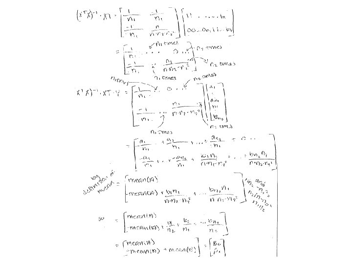
With “A” as the background…. = B 0 + B 1 + Extra credit: Prove in general for the above model that B 0 = mean(A) and B 1 = mean(B)- mean(A)

Proof! From Brittany Smith and then…

Next: Towards multivariate models. One WAY-Anova with multiple levels. Combining regression and t-test (Analysis of covariance) Multiple ANOVAs and regressions (with interaction terms) Using Principle Component Analysis (PCA) to attack multi-dimensional data