Matrix Factorization Singular Value Decomposition Bamshad Mobasher De

Matrix Factorization & Singular Value Decomposition Bamshad Mobasher De. Paul University

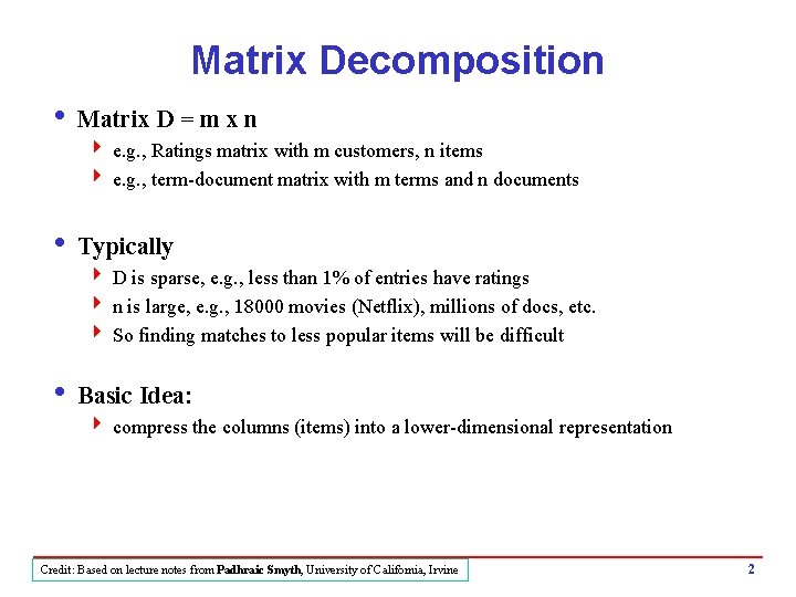
Matrix Decomposition i Matrix D = m x n 4 e. g. , Ratings matrix with m customers, n items 4 e. g. , term-document matrix with m terms and n documents i Typically 4 D is sparse, e. g. , less than 1% of entries have ratings 4 n is large, e. g. , 18000 movies (Netflix), millions of docs, etc. 4 So finding matches to less popular items will be difficult i Basic Idea: 4 compress the columns (items) into a lower-dimensional representation Credit: Based on lecture notes from Padhraic Smyth, University of California, Irvine 2

Singular Value Decomposition (SVD) D m where: x S Vt = U n m x n n x n rows of Vt are eigenvectors of Dt. D = basis functions S is diagonal, with sii = sqrt(li) (ith eigenvalue) rows of U are coefficients for basis functions in V (here we assumed that m > n, and rank(D) = n) Credit: Based on lecture notes from Padhraic Smyth, University of California, Irvine 3

Singular Value Decomposition (SVD) where: rows of Vt are eigenvectors of Dt. D = basis functions S is diagonal, with sii = sqrt(li) (ith eigenvalue) rows of U are coefficients for basis functions in V (here we assumed that m > n, and rank(D) = n) Credit: Based on lecture notes from Padhraic Smyth, University of California, Irvine 4

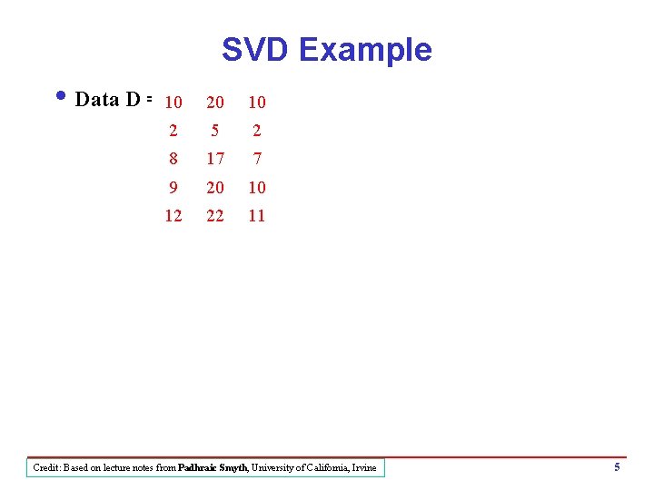
SVD Example i Data D = 10 20 10 2 5 2 8 17 7 9 20 10 12 22 11 Credit: Based on lecture notes from Padhraic Smyth, University of California, Irvine 5

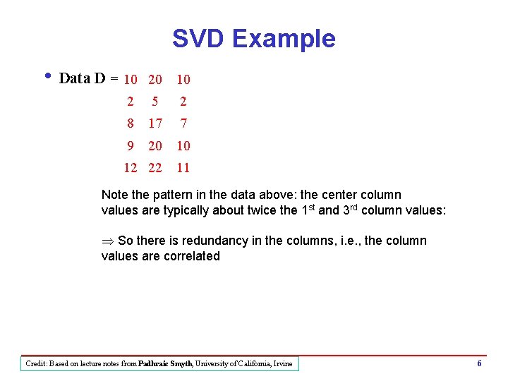
SVD Example i Data D = 10 20 10 2 5 2 8 17 7 9 20 10 12 22 11 Note the pattern in the data above: the center column values are typically about twice the 1 st and 3 rd column values: Þ So there is redundancy in the columns, i. e. , the column values are correlated Credit: Based on lecture notes from Padhraic Smyth, University of California, Irvine 6

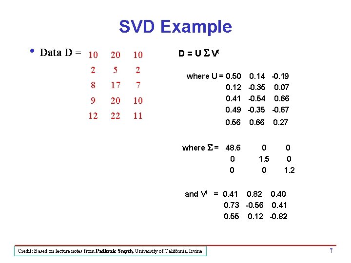
SVD Example i Data D = 10 20 10 2 5 2 8 17 7 9 20 10 12 22 11 D = U S Vt where U = 0. 50 0. 14 -0. 19 0. 12 -0. 35 0. 07 0. 41 -0. 54 0. 66 0. 49 -0. 35 -0. 67 0. 56 where S = 48. 6 0 0 0. 66 0 1. 5 0 0. 27 0 0 1. 2 and Vt = 0. 41 0. 82 0. 40 0. 73 -0. 56 0. 41 0. 55 0. 12 -0. 82 Credit: Based on lecture notes from Padhraic Smyth, University of California, Irvine 7

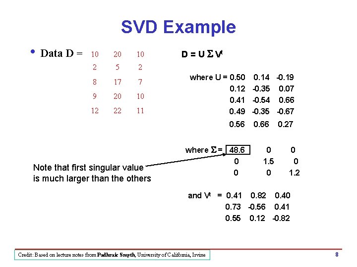
SVD Example i Data D = 10 20 10 2 5 2 8 17 7 9 20 10 12 22 11 D = U S Vt where U = 0. 50 0. 14 -0. 19 0. 12 -0. 35 0. 07 0. 41 -0. 54 0. 66 0. 49 -0. 35 -0. 67 0. 56 Note that first singular value is much larger than the others where S = 48. 6 0 0 0. 66 0 1. 5 0 0. 27 0 0 1. 2 and Vt = 0. 41 0. 82 0. 40 0. 73 -0. 56 0. 41 0. 55 0. 12 -0. 82 Credit: Based on lecture notes from Padhraic Smyth, University of California, Irvine 8

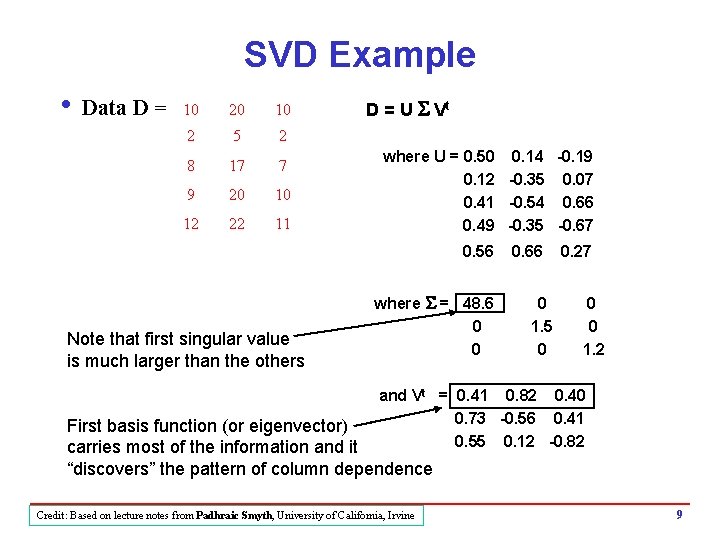
SVD Example i Data D = 10 20 10 2 5 2 8 17 7 9 20 10 12 22 11 D = U S Vt where U = 0. 50 0. 14 -0. 19 0. 12 -0. 35 0. 07 0. 41 -0. 54 0. 66 0. 49 -0. 35 -0. 67 0. 56 Note that first singular value is much larger than the others where S = 48. 6 0 0 0. 66 0 1. 5 0 0. 27 0 0 1. 2 and Vt = 0. 41 0. 82 0. 40 0. 73 -0. 56 0. 41 0. 55 0. 12 -0. 82 First basis function (or eigenvector) carries most of the information and it “discovers” the pattern of column dependence Credit: Based on lecture notes from Padhraic Smyth, University of California, Irvine 9

Rows in D = weighted sums of basis vectors 1 st row of D = [10 20 10] Since D = U S Vt , then D[0, : ] = U[0, : ] * S * Vt = [24. 5 0. 2 -0. 22] * Vt Vt = 0. 41 0. 82 0. 40 0. 73 -0. 56 0. 41 0. 55 0. 12 -0. 82 Þ D[0, : ] = 24. 5 v 1 + 0. 2 v 2 + -0. 22 v 3 where v 1 , v 2 , v 3 are rows of Vt and are our basis vectors Thus, [24. 5, 0. 22] are the weights that characterize row 1 in D In general, the ith row of U* S is the set of weights for the ith row in D Credit: Based on lecture notes from Padhraic Smyth, University of California, Irvine 10

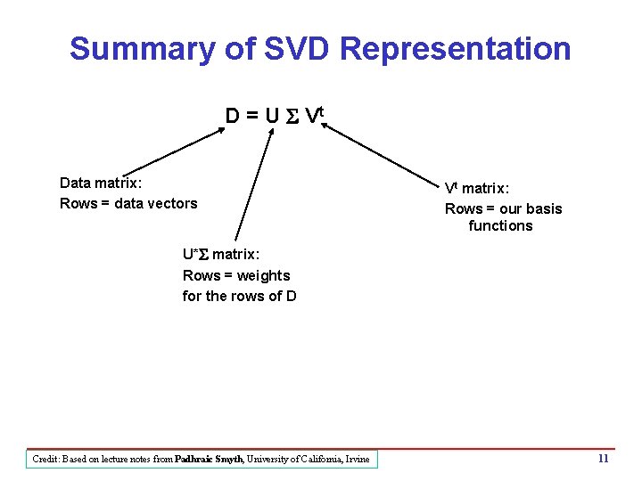
Summary of SVD Representation D = U S Vt Data matrix: Rows = data vectors Vt matrix: Rows = our basis functions U*S matrix: Rows = weights for the rows of D Credit: Based on lecture notes from Padhraic Smyth, University of California, Irvine 11

How do we compute U, S, and V? i SVD decomposition is a standard eigenvector/value problem 4 The eigenvectors of Dt * D = the rows of V 4 The eigenvectors of D * Dt = the columns of U 4 The diagonal matrix elements in S are square roots of the eigenvalues of Dt * D => finding U, S, V is equivalent to finding eigenvectors of Dt. D 4 Solving eigenvalue problems is equivalent to solving a set of linear equations – time complexity is O(m n 2 + n 3) Credit: Based on lecture notes from Padhraic Smyth, University of California, Irvine 12

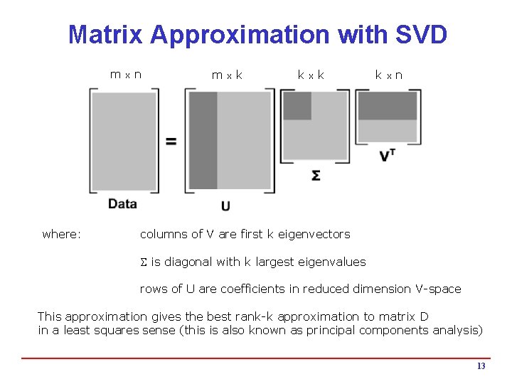
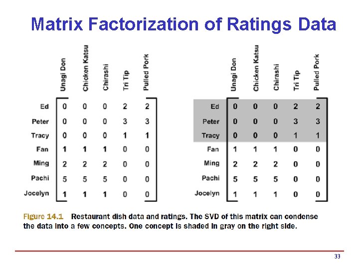
Matrix Approximation with SVD m where: x n m x k k x n columns of V are first k eigenvectors S is diagonal with k largest eigenvalues rows of U are coefficients in reduced dimension V-space This approximation gives the best rank-k approximation to matrix D in a least squares sense (this is also known as principal components analysis) 13

Recommendation as Rating Prediction i Two types of entities: Users and Items i Utility of item i for user u is represented by some rating r (where r ∈ Rating) could be explicit or implicit i Each user typically rates a subset of items i Recommender system then tries to estimate the unknown ratings, i. e. , to extrapolate rating function R based on the known ratings: 4 R: Users × Items → Rating i The recommendations to each user are made by offering items with highest predicted rating 14

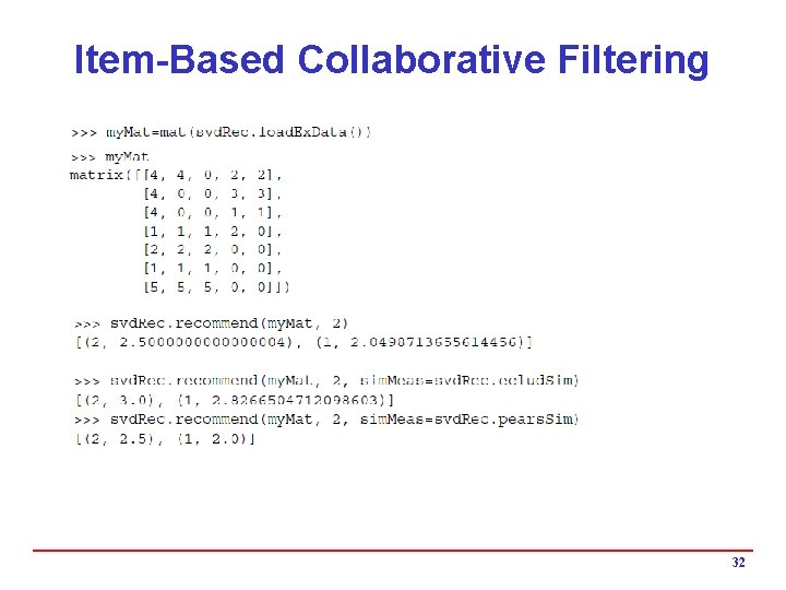
Collaborative Recommender Systems Neighborhood-Based Models i User-Based: 4 For a target user u, find the top k most similar users (based on their rating profiles) who have rated the target item 4 k-nearest-neighbor (knn) strategy 4 Predicted rating on target item is weighted average of ratings by the neighbors. i Item-based Collaborative Filtering 4 item-item similarities are computed in space of ratings itwo items are similar if they are rated similarly by users 4 prediction for target item is computed based on user u’s own ratings on the k most similar items

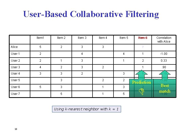
User-Based Collaborative Filtering Item 1 Item 2 Item 3 Item 4 Alice 5 2 3 3 User 1 2 User 2 2 User 3 User 4 User 7 Correlation with Alice ? 4 1 -1. 00 1 3 1 2 0. 33 4 2 3 1 . 90 3 3 2 1 0. 19 2 -1. 00 5 2 3 3 2 2 3 1 3 5 1 5 Using k-nearest neighbor with k = 1 16 Item 6 4 User 5 User 6 Item 5 Prediction 2 1 Best 0. 65 match -1. 00

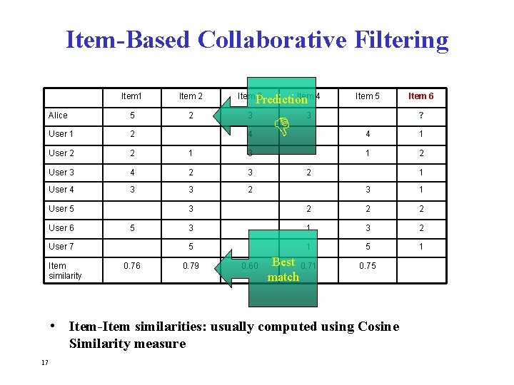
Item-Based Collaborative Filtering Item 1 Item 2 Item 3 Alice 5 2 3 User 1 2 User 2 2 1 3 User 3 4 2 3 User 4 3 3 2 User 5 User 6 5 User 7 Item similarity 0. 76 Item 4 Prediction 4 Item 5 3 ? 4 1 1 2 2 1 3 2 2 2 3 1 3 2 5 1 0. 79 0. 60 Best 0. 71 match 0. 75 • Item-Item similarities: usually computed using Cosine Similarity measure 17 Item 6

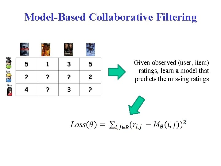
Model-Based Collaborative Filtering Given observed (user, item) ratings, learn a model that predicts the missing ratings

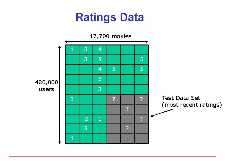
Collaborative Filtering & Matrix Factorization 17, 700 movies 1 3 4 3 5 4 The $1 Million Question 5 5 5 2 2 3 480, 000 users 3 2 5 2 3 1 1 1 3

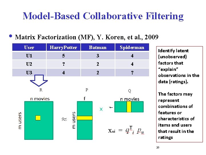
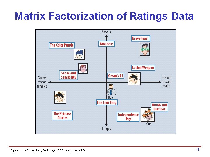
Model-Based Collaborative Filtering i Matrix Factorization (MF), Y. Koren, et al. , 2009 User Harry. Potter Batman Spiderman U 1 5 3 4 U 2 ? 2 4 U 3 4 2 ? R P Q Identify latent (unobserved) factors that “explain” observations in the data (ratings). The factors may represent combinations of features or characteristics of items and users that result in the ratings 20

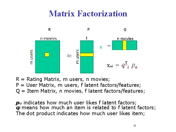
Matrix Factorization R P Q R = Rating Matrix, m users, n movies; P = User Matrix, m users, f latent factors/features; Q = Item Matrix, n movies, f latent factors/features; pu indicates how much user likes f latent factors; qi means how much an item is related to f latent factors; The dot product indicates how much user likes item; 21

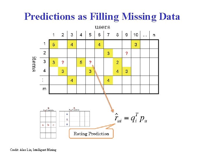
Predictions as Filling Missing Data Credit: Alex Lin, Intelligent Mining

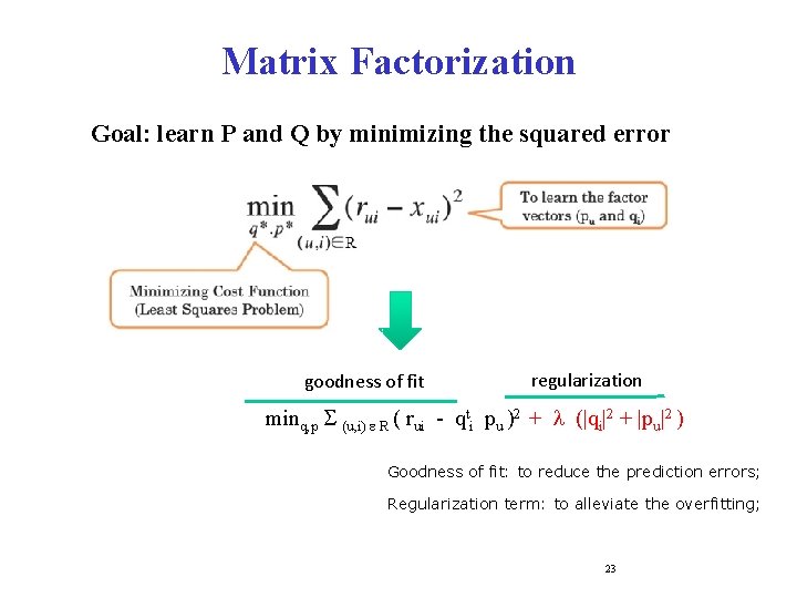
Matrix Factorization Goal: learn P and Q by minimizing the squared error goodness of fit regularization minq, p S (u, i) e R ( rui - qti pu )2 + l (|qi|2 + |pu|2 ) Goodness of fit: to reduce the prediction errors; Regularization term: to alleviate the overfitting; 23

Matrix Factorization Goal: learn P and Q by minimizing the squared error goodness of fit regularization minq, p S (u, i) e R ( rui - qti pu )2 + l (|qi|2 + |pu|2 ) By using Stochastic Gradient Descent (SGD) or Alternating Least Squares (ALS), we are able to learn the P and Q iteratively.

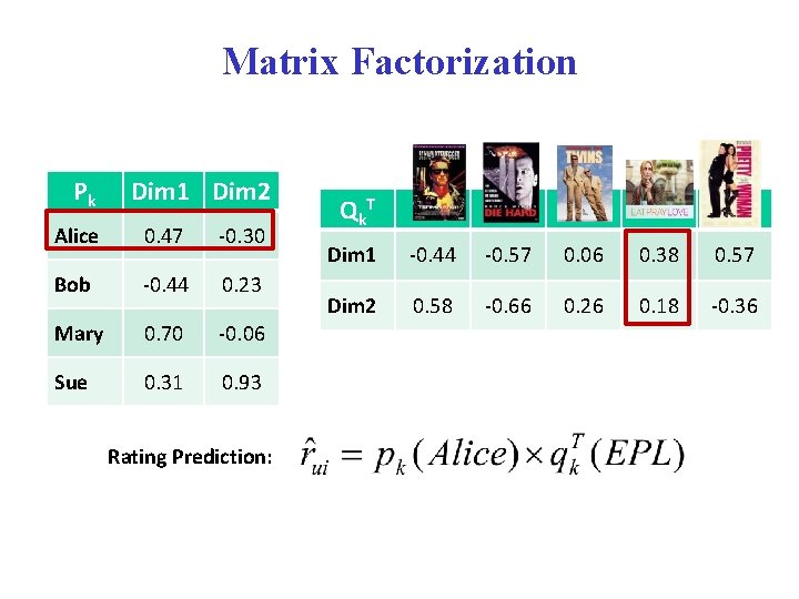
Matrix Factorization Pk Dim 1 Dim 2 Alice 0. 47 -0. 30 Bob -0. 44 0. 23 Mary 0. 70 -0. 06 Sue 0. 31 0. 93 Rating Prediction: Qk T Dim 1 -0. 44 -0. 57 0. 06 0. 38 0. 57 Dim 2 0. 58 -0. 66 0. 26 0. 18 -0. 36

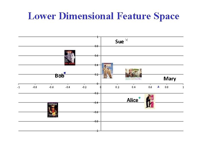
Lower Dimensional Feature Space 1 Sue 0. 8 0. 6 0. 4 Bob 0. 2 Mary 0 -1 -0. 8 -0. 6 -0. 4 -0. 2 0. 4 -0. 2 -0. 4 -0. 6 -0. 8 -1 Alice 0. 6 0. 8 1

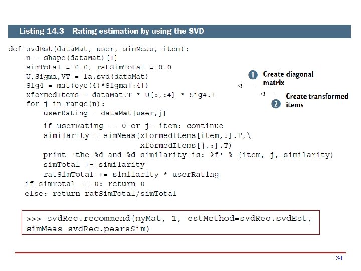
SVD for Matrix Factorization We can also do factorization via Singular Value Decomposition (SVD), by reducing to top k singular values: In this case, Uk represents the user-feature matrix and Vk. T represents the feature-item matrix. Rating predictions can be computed as before using dot products. Uk Dim 1 Dim 2 Alice 0. 47 -0. 30 Bob -0. 44 0. 23 Mary 0. 70 -0. 06 Sue 0. 31 0. 93 Vk T Dim 1 -0. 44 -0. 57 0. 06 0. 38 0. 57 Dim 2 0. 58 -0. 66 0. 26 0. 18 -0. 36

Evaluation: Rating Prediction User Item Rating U 1 T 1 4 U 1 T 2 3 U 1 T 3 3 U 2 T 2 4 U 2 T 3 5 U 2 T 4 5 U 3 T 4 4 U 1 T 4 3 U 2 T 1 2 U 3 T 2 3 U 3 T 3 4 P(U, T) in testing set Prediction error: Train e = R(U, T) – P(U, T) Mean Absolute Error (MAE) = Test Other evaluation metrics: • Root Mean Square Error (RMSE) • Coverage • many more …

MLA Book; Ch. 14 – svd. Rec. py First three values are much larger than the rest 29

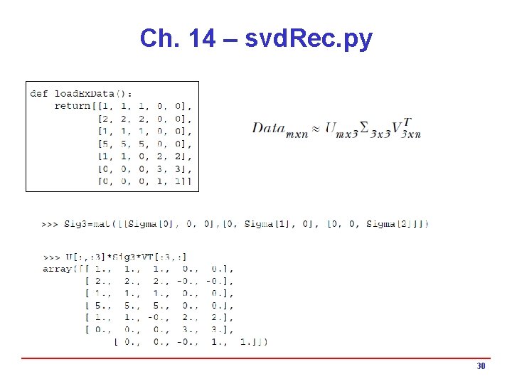
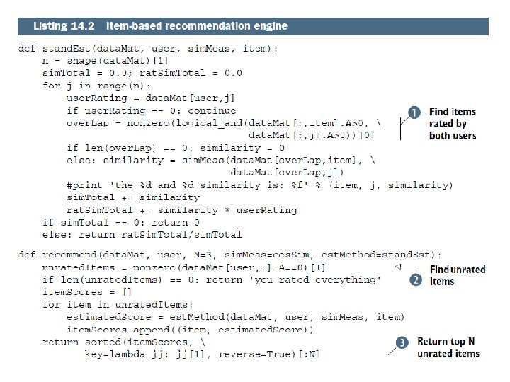
Ch. 14 – svd. Rec. py 30

31

Item-Based Collaborative Filtering 32

Matrix Factorization of Ratings Data 33

34

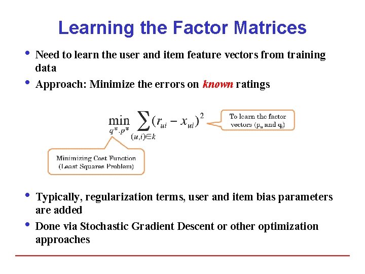
Learning the Factor Matrices i Need to learn the user and item feature vectors from training data i Approach: Minimize the errors on known ratings i Typically, regularization terms, user and item bias parameters are added i Done via Stochastic Gradient Descent or other optimization approaches

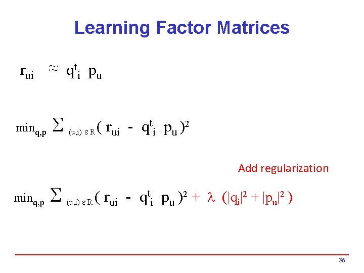
Learning Factor Matrices ~ qti pu rui ~ minq, p S t p )2 ( r q (u, i) e R ui i u Add regularization minq, p S t p )2 + l (|q |2 + |p |2 ) ( r q (u, i) e R i u ui i u 36

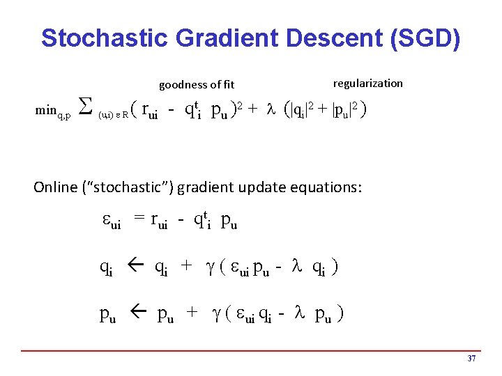
Stochastic Gradient Descent (SGD) minq, p S goodness of fit regularization t p )2 + l (|q |2 + |p |2 ) ( r q (u, i) e R i u ui i u Online (“stochastic”) gradient update equations: eui = rui - qti pu qi + g ( eui pu - l qi ) pu + g ( eui qi - l pu ) 37

The $1 Million Question 38

Training Data i 100 million ratings (matrix is 99% sparse) i Rating = [user, movie-id, time-stamp, rating value] i Generated by users between Oct 1998 and Dec 2005 i Users randomly chosen among set with at least 20 ratings 4 Small perturbations to help with anonymity 39

Ratings Data 17, 700 movies 1 3 4 3 5 4 5 5 5 ? ? 3 480, 000 users 3 2 ? 2 3 1 1 ? ? Test Data Set (most recent ratings)

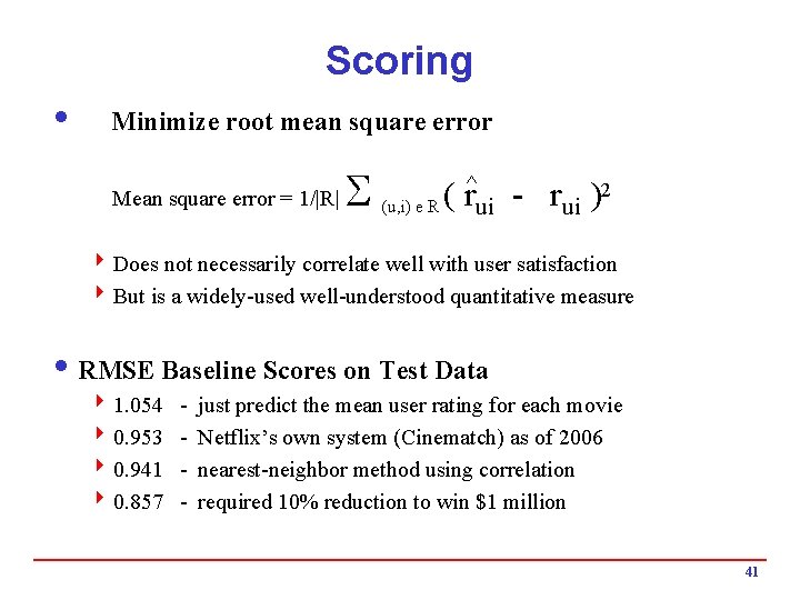
Scoring i Minimize root mean square error Mean square error = 1/|R| S ^ 2 ( r r ) (u, i) e R ui ui 4 Does not necessarily correlate well with user satisfaction 4 But is a widely-used well-understood quantitative measure i RMSE Baseline Scores on Test Data 4 1. 054 4 0. 953 4 0. 941 4 0. 857 - just predict the mean user rating for each movie Netflix’s own system (Cinematch) as of 2006 nearest-neighbor method using correlation required 10% reduction to win $1 million 41

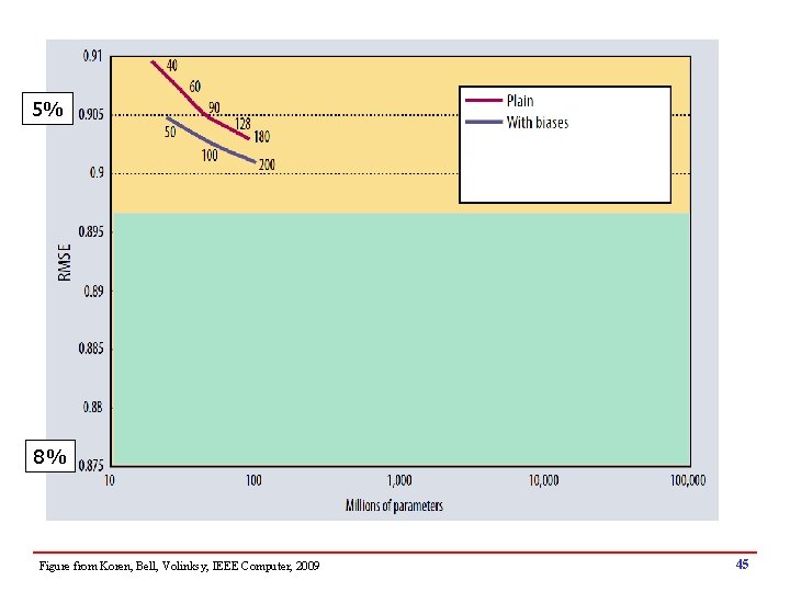
Matrix Factorization of Ratings Data Figure from Koren, Bell, Volinksy, IEEE Computer, 2009 42

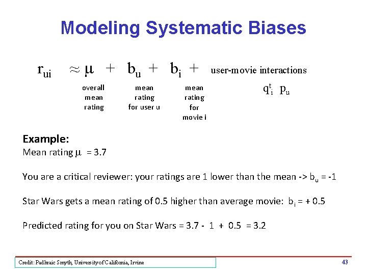
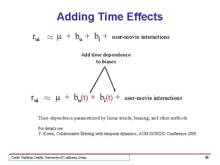
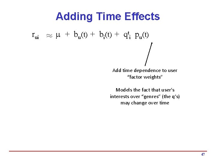
Modeling Systematic Biases rui ~ ~ m + bu + bi + overall mean rating for user u mean rating for movie i user-movie interactions qti pu Example: Mean rating m = 3. 7 You are a critical reviewer: your ratings are 1 lower than the mean -> bu = -1 Star Wars gets a mean rating of 0. 5 higher than average movie: bi = + 0. 5 Predicted rating for you on Star Wars = 3. 7 - 1 + 0. 5 = 3. 2 Credit: Padhraic Smyth, University of California, Irvine 43

Objective Function minq, p {S goodness of fit (u, i) e R ( rui - (m + bu + bi + qti pu ) )2 + l (|qi|2 + |pu|2 + |bi|2 ) } regularization Typically selected via grid-search on a validation set Credit: Padhraic Smyth, University of California, Irvine 44

5% 8% Figure from Koren, Bell, Volinksy, IEEE Computer, 2009 45

Adding Time Effects rui ~ ~ m + bu + bi + user-movie interactions Add time dependence to biases rui ~ m + bu(t) + bi(t) + user-movie interactions Time-dependence parametrized by linear trends, binning, and other methods For details see Y. Koren, Collaborative filtering with temporal dynamics, ACM SIGKDD Conference 2009 Credit: Padhraic Smyth, University of California, Irvine 46

Adding Time Effects t p (t) rui ~ m + b (t) + q u i i u ~ Add time dependence to user “factor weights” Models the fact that user’s interests over “genres” (the q’s) may change over time 47

5% 8% Figure from Koren, Bell, Volinksy, IEEE Computer, 2009 48

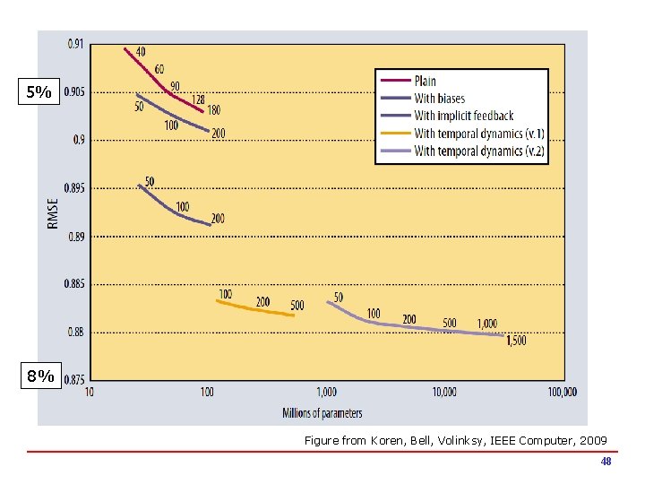
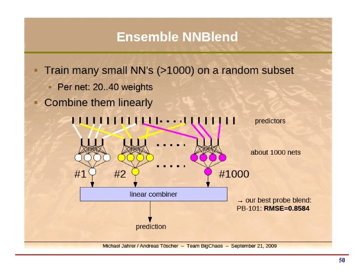
The Kitchen Sink Approach…. i Many options for modeling 4 Variants of the ideas we have seen so far h Different numbers of factors h Different ways to model time h Different ways to handle implicit information h …. 4 Other models (not described here) h Nearest-neighbor models h Restricted Boltzmann machines i Model averaging was useful…. 4 Linear model combining 4 Neural network combining 4 Gradient boosted decision tree combining 4 Note: combining weights learned on validation set (“stacking”) Credit: Padhraic Smyth, University of California, Irvine 49

50

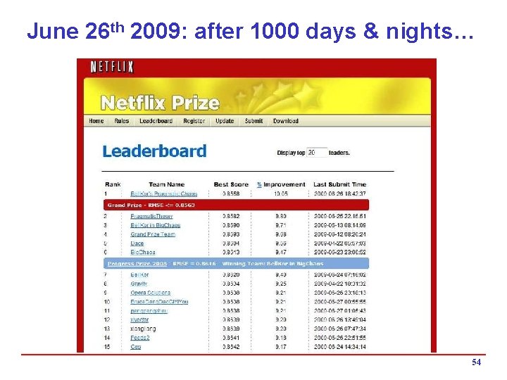
Progress Prize 2008 Sept 2 nd Only 3 teams qualify for 1% improvement over previous year Oct 2 nd Leading team has 9. 4% overall improvement Progress prize ($50, 000) awarded to Bell. Kor team of 3 AT&T researchers (same as before) plus 2 Austrian graduate students, Andreas Toscher and Martin Jahrer Key winning strategy: clever “blending” of predictions from models used by both teams Speculation that 10% would be attained by mid-2009 51

The Leading Team for the Final Prize i. Bell. Kor. Pragmatic. Chaos 4 Bell. Kor: h. Yehuda Koren (now Yahoo!), Bob Bell, Chris Volinsky, AT&T 4 Big. Chaos: h Michael Jahrer, Andreas Toscher, 2 grad students from Austria 4 Pragmatic Theory h. Martin Chabert, Martin Piotte, 2 engineers from Montreal (Quebec) 52

53

June 26 th 2009: after 1000 days & nights… 54

Million Dollars Awarded Sept 21 st 2009 55