Matrix exponent Using stable numeric algorithm Teddy Lazebnik

Agenda › Motivation to solve matrix exponent › Definition of the problem › Known algorithm and the original Lanzos & Putzer algorithms › The improvement › Choose tree algorithm › Numerical results › Example of real world application

Motivation to solve matrix exponent Matrix exponent can be found in many areas of applied mathematics, for example: In control theory, A linear control system with continues time measurement described by O. D. E. When the system is presented as a combination of smaller systems it describes as a vector and the mathematical model describes such systems is a matrix exponent. Other example can be the ability to convert continuous-time system into discrete-time state-space system.

Motivation to solve matrix exponent When looking on a robotic system mimics the walking process of a person we can describe the dynamics of the system by a discrete – continues function described by continues ODE of space, time when the “foot” of the robot is in the air and a shock functions when making a “step” on the ground. To make sure the robot is not falling as a result of the noise in a real world system; one can use a control system to supervise the right operation of the robot. These systems use several sensors to retrieve the information but putting sensor and analyze it’s signal on all the needed parameters is costly and not efficient technic.

Motivation to solve matrix exponent Control system uses a part group of the sensors which satisfices the observable condition. The observable condition stands for that we can retrieve the full system information based on the partial group. The process of calculating the observer of a system uses matrix exponent. An unstable calculation of the matrix exponent bubbles to the calculation of the observer and decide the effectiveness of the control system.

Matrix exponent Forms Differential system Interpolation Cauchy integral Padé approximation Power series Limit

Matrix exponent properties ›

Definitions ›

Definitions – examples

Problem’s definition ›

Known algorithms P’ade approximation based method Cayley–Hamilton based method

Known algorithms Lagrange interpolation based method Newton interpolation based method

Known algorithms Inverse Laplace transforms based method General purpose O. D. E. solver This is not a specific algorithm. It’s based on the idea that calculate the result of the following equation with O. D. E solves algorithms will produce the right answer;

Unstable algorithm example ›

The original solution E. J. Putzer lived in Germany at the 20 th century, he was an engineer and published the “Avoiding the Jordan canonical form in the discussion of linear systems with constant coefficients” Cornelius Lanczos lived in Hungary. Born at 1893 and died at 1974, he was a mathematician and physicist and work on many fields of applied mathematics. E. J. Putzer Cornelius Lanczos

Putzer’s algorithm ›

Putzer’s algorithm proof ›

Lanczos’ algorithm ›

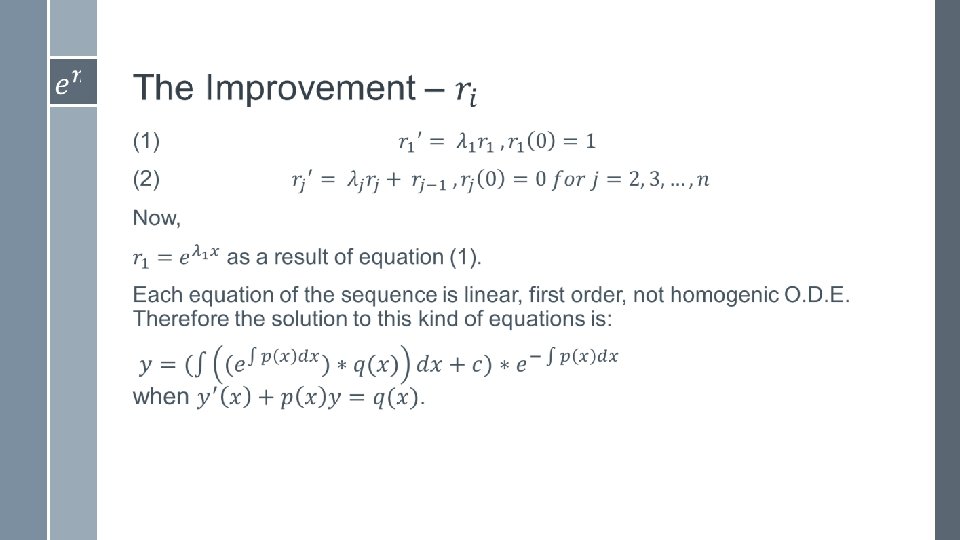
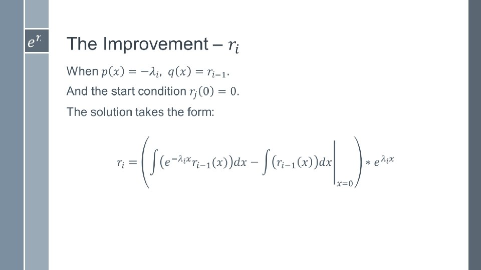
The Improvement ›

The Improvement - Lemma 1 ›

The Improvement - Lemma 2 ›

Examples ›

Stability of the algorithm ›

Numerical analysis ›

Storage requirements ›

Complexity ›

Comparison with other algorithms ›

Comparison with other algorithms case 1 case 2 case 3 case 4 case 5 case 6 case 7 case 8 Naive 0. 01 1. 09 Error O(10^-14) Error Pad 9. 34 3. 42 Error 23. 19 Error 6. 03 35. 92 155. 98 Newton 5. 38 2. 38 Error 17. 08 Error 2. 98 182. 74 143. 41 Lagrange 0. 01 1. 09 Error 20. 08 Error 4. 48 78. 46 Teddy 0. 07 0. 98 Error O(10^-15) Error 133. 81 148. 41

Comparison with other algorithms case 1 Naive 1. 63 Pad 37. 37 case 2 case 3 case 4 case 5 case 6 case 7 0. 10 Error 65. 59 Error 5. 47 1. 88 Error 9. 49 Error 37. 01 7. 94 8. 92 29. 61 45. 30 7. 13 Newton 29. 97 1. 07 Error 8. 47 Error Lagrange 0. 45 0. 05 Error 5. 27 Error 8. 17 5. 55 Teddy 0. 32 0. 65 Error 2. 37 Error 12. 05 13. 06

Comparison with other algorithms case 1 case 2 case 3 case 4 case 5 case 6 case 7 Naive 1. 63 0. 10 Error 65. 59 Error Pad 4. 67 1. 84 Error 48. 61 Error 0. 76 168. 17 58. 79 Newton 2. 58 1. 02 Error 47. 88 Error 1. 43 319. 22 57. 56 Lagrange 1. 637 0. 10 Error 3. 42 193. 18 Teddy 1. 42 0. 06 Error 38. 19 Error 72. 58 541. 01 112. 90

Decision tree algorithm The new algorithm presented is stable but not the most effective in most of the cases. Therefore, we developed an algorithm which preservative stability and trying to improve efficiency as much as possible… The algorithm based on a choosing tree when the leafs are algorithms for matrix exponent and the other nodes operates as a condition – state for the matrix.

Choose tree algorithm – structure

Choose tree algorithm – Compare case 1 case 2 case 3 case 4 Decision tree 0. 07 2. 38 Not E E Best result 0. 01 1. 09 E E Match? no no Yes case 6 0 133. 81 case 7 35. 92 Yes case 1 case 2 case 3 0. 32 1. 07 Not E 2. 37 E Best result 0. 32 0. 05 E 2. 37 E Match? Yes No Yes Yes case 1 case 2 case 3 1. 42 1. 02 Not E 38. 19 E Best result 1. 42 0. 06 E 38. 19 E Match? Yes No Yes Yes Decision case 5 case 4 Yes No Yes case 5 case 6 case 7 0 12. 05 5. 47 7. 94 5. 47 No Yes tree Decision case 4 Yes case 5 case 6 case 7 0 541. 01 112. 90 168. 17 57. 56 No no tree Yes The decision tree gets the best result 16 out of 24 cases. This decision tree algorithm is 67% of the time the best choice for EXPM.

Example to real world application

References › [1] R. M. Karp, "Reducibility among Combinatorial Problems", Complexity of Computer Computations, (1972), pp. 85 -103. › [2] Erik Wahlén, “Alternative proof of Putzer’s algorithm”, (2013) (http: //www. ctr. maths. lu. se/media/MATM 14/2013 vt 2013/putzer. p df) › [3] James Demmel, Ioana Dumitriu, Olga Holtz, and Robert Kleinberg, “Fast matrix multiplication is stable”, (2006) (https: //www. math. washington. edu/~dumitriu/fmm_arxiv. pdf ) › [4] Grigory Agranovich, Ariel University, ” Observer for Discrete. Continuous LTI with continuous-time measurements” (2010)

References › [5] Cleve Moler, Charles Van Loan, Society for Industrial and Applied Mathematics, “Nineteen Dubious Ways to Compute the Exponential of a Matrix, Twenty-Five Years Later” (2003) › [6] Lanczos, C. "An iteration method for the solution of the eigenvalue problem of linear differential and integral operators", J. Res. Nat’l Bur. Std. 45, 225 -282 (1950). › [7] Ojalvo, I. U. and Newman, M. , "Vibration modes of large structures by an automatic matrix-reduction method", AIAA J. , 8 (7), 1234– 1239 (1970). › [8] Trefethen, Lloyd N. ; Bau, David, Numerical linear algebra, Philadelphia: Society for Industrial and Applied Mathematics, ISBN 978 -0 -89871 -361 -9 (1997)

Implementation An example of Matlab code which run this algorithm is: function [ expm ] = expm_stable( M ) Roots = eigs(M); syms x; r = exp(Roots(1)*x); p = eye(size(M)); Y = r * p; for i = 2: (size(Roots, 1)) r = (int((exp((-1)*Roots(i)*x))*r)subs(int(r), x, 0))*exp(Roots(i)*x); p = p * (M - Roots(i)*eye(size(M))); Y = Y + r * p; end expm = subs(Y, x, 1); end This code is not numeric, it uses a symbolic calculation

Implementation Numeric implementation in C#: Matrix_Ri 2 dim array of Ri Ri List of Expoly List of double Single double

Implementation The all code is long and out of the scope of this desiccation, I will present only the top function: public Matrix. Ri Expm(double[, ] original. Matrix, double[] eigs) { Matrix. Ri exp. M = new Matrix. Ri(original. Matrix. Get. Length(0)); Matrix. Ri p = new Matrix. Ri(eye(exp. M. elements. Get. Length(0))); Ri ri = new Ri(); ri = ri. mult. Exp(eigs[0]); for (int i = 0; i < exp. M. elements. Get. Length(0); i++) { exp. M. elements[i, i] = ri; } for (int i = 1; i < exp. M. elements. Get. Length(0); i++) { ri = ri. do. Step(eigs[i]); p = p. mult(sub. Matrix(original. Matrix, eye(eigs. Length, eigs[i]))); exp. M = exp. M. Addition(p. mult. Ri(ri)); } return exp. M; }