Matrix Diagonalisation Diagonalization of matrices is very easy

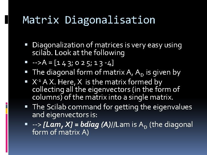
Matrix Diagonalisation Diagonalization of matrices is very easy using scilab. Look at the following -->A = [1 4 3; 0 2 5; 1 3 -4] The diagonal form of matrix A, AD is given by X-1 A X. Here, X is the matrix formed by collecting all the eigenvectors (in the form of columns) of the matrix into a single matrix. The Scilab command for getting the eigenvalues and eigenvectors is: --> [Lam, X] = bdiag (A)//Lam is AD (the diagonal form of matrix A)

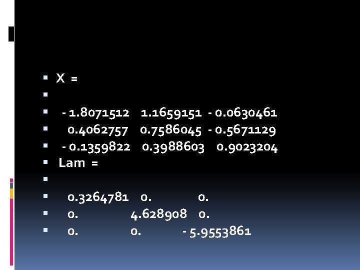
X = - 1. 8071512 1. 1659151 - 0. 0630461 0. 4062757 0. 7586045 - 0. 5671129 - 0. 1359822 0. 3988603 0. 9023204 Lam = 0. 3264781 0. 0. 0. 4. 628908 0. 0. 0. - 5. 9553861

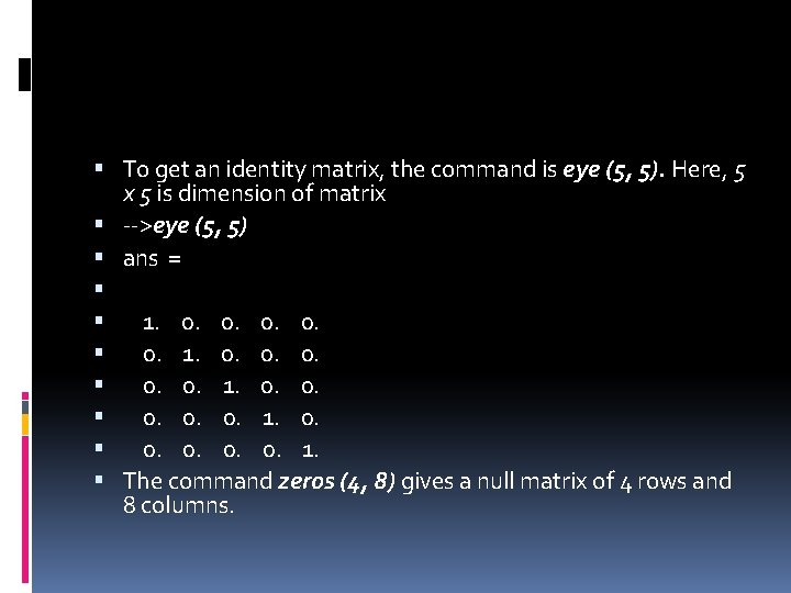
To get an identity matrix, the command is eye (5, 5). Here, 5 x 5 is dimension of matrix -->eye (5, 5) ans = 1. 0. 0. 0. 1. 0. 0. 1. The command zeros (4, 8) gives a null matrix of 4 rows and 8 columns.

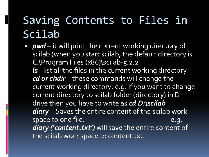
Saving Contents to Files in Scilab pwd – it will print the current working directory of scilab (when you start scilab, the default directory is C: Program Files (x 86)scilab-5. 2. 2 ls - list all the files in the current working directory cd or chdir – these commands will change the current working directory. e. g. if you want to change current directory to scilab folder (directory) in D drive then you have to write as cd D: scilab diary – Saves the entire content of the scilab work space to one file. e. g. diary (‘content. txt’) will save the entire content of the scilab work space to content. txt.

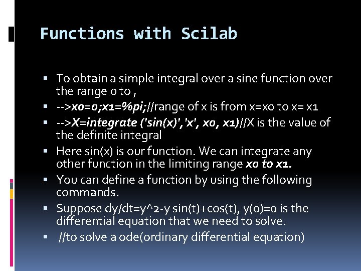
Functions with Scilab To obtain a simple integral over a sine function over the range 0 to , -->x 0=0; x 1=%pi; //range of x is from x=x 0 to x= x 1 -->X=integrate ('sin(x)', 'x', x 0, x 1)//X is the value of the definite integral Here sin(x) is our function. We can integrate any other function in the limiting range x 0 to x 1. You can define a function by using the following commands. Suppose dy/dt=y^2 -y sin(t)+cos(t), y(0)=0 is the differential equation that we need to solve. //to solve a ode(ordinary differential equation)

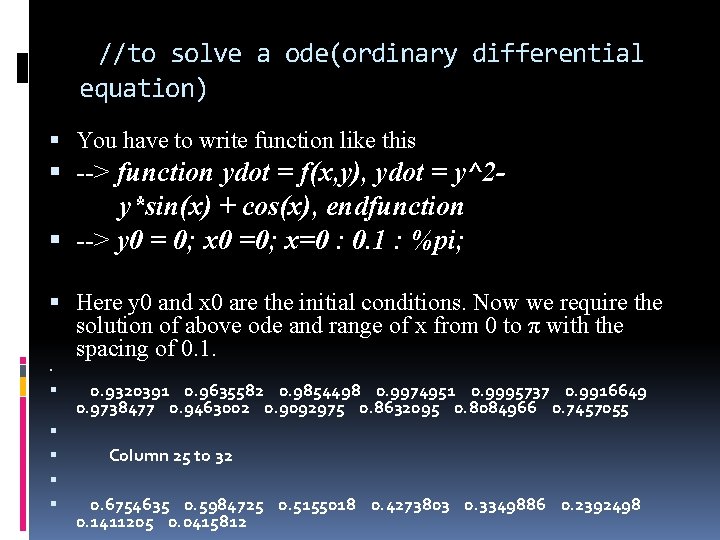
//to solve a ode(ordinary differential equation) You have to write function like this --> function ydot = f(x, y), ydot = y^2 y*sin(x) + cos(x), endfunction --> y 0 = 0; x 0 =0; x=0 : 0. 1 : %pi; Here y 0 and x 0 are the initial conditions. Now we require the solution of above ode and range of x from 0 to π with the spacing of 0. 1. 0. 9320391 0. 9635582 0. 9854498 0. 9974951 0. 9995737 0. 9916649 0. 9738477 0. 9463002 0. 9092975 0. 8632095 0. 8084966 0. 7457055 Column 25 to 32 0. 6754635 0. 5984725 0. 5155018 0. 4273803 0. 3349886 0. 2392498 0. 1411205 0. 0415812

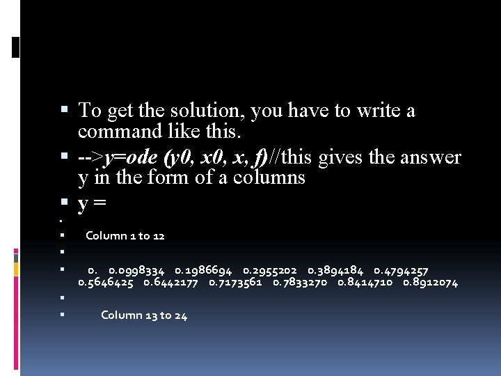
To get the solution, you have to write a command like this. -->y=ode (y 0, x, f)//this gives the answer y in the form of a columns y= Column 1 to 12 0. 0. 0998334 0. 1986694 0. 2955202 0. 3894184 0. 4794257 0. 5646425 0. 6442177 0. 7173561 0. 7833270 0. 8414710 0. 8912074 Column 13 to 24

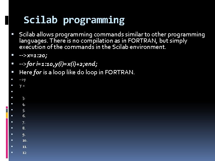
Scilab programming Scilab allows programming commands similar to other programming languages. There is no compilation as in FORTRAN, but simply execution of the commands in the Scilab environment. -->x=1: 20; -->for i=1: 10, y(i)=x(i)+2; end; Here for is a loop like do loop in FORTRAN. -->y y= 3. 4. 5. 6. 7. 8. 9. 10. 11. 12