Matrix Computation n Multiple Regression n Generalized Linear

矩陣運算(Matrix Computation) 矩陣運算在統計分析上扮演非常重要的角 色，包括以下方法： n Multiple Regression n Generalized Linear Model n Multivariate Analysis n Time Series n Other topics (Random variables)

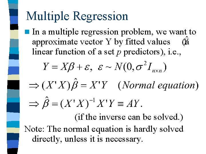
Multiple Regression n In a multiple regression problem, we want to approximate vector Y by fitted values (a linear function of a set p predictors), i. e. , (if the inverse can be solved. ) Note: The normal equation is hardly solved directly, unless it is necessary.

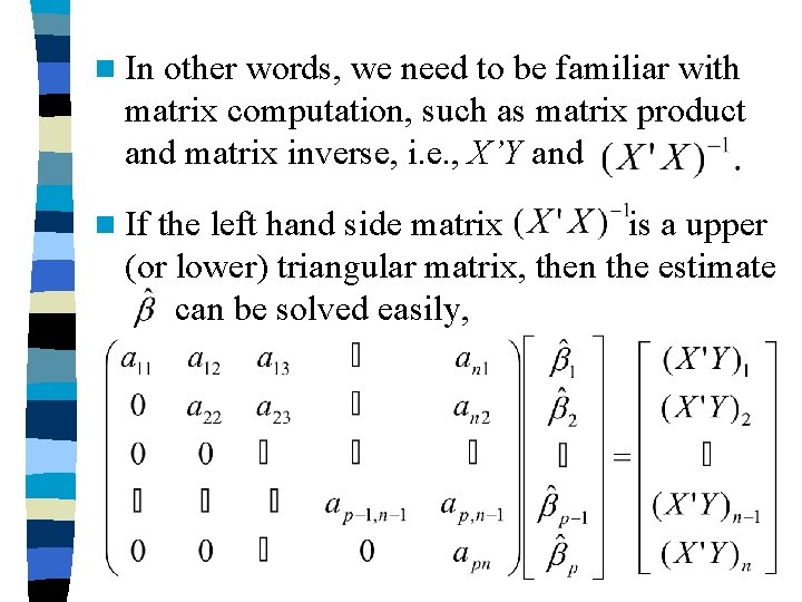
n In other words, we need to be familiar with matrix computation, such as matrix product and matrix inverse, i. e. , X’Y and n If the left hand side matrix is a upper (or lower) triangular matrix, then the estimate can be solved easily,

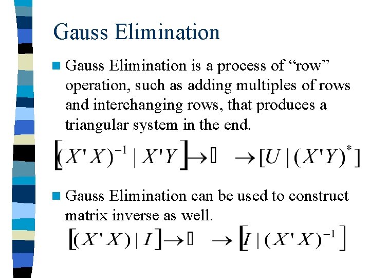
Gauss Elimination n Gauss Elimination is a process of “row” operation, such as adding multiples of rows and interchanging rows, that produces a triangular system in the end. n Gauss Elimination can be used to construct matrix inverse as well.

n An Example of Gauss Elimination:

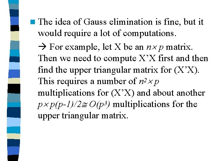
n The idea of Gauss elimination is fine, but it would require a lot of computations. For example, let X be an n p matrix. Then we need to compute X’X first and then find the upper triangular matrix for (X’X). This requires a number of n 2 p multiplications for (X’X) and about another p p(p-1)/2 O(p 3) multiplications for the upper triangular matrix.

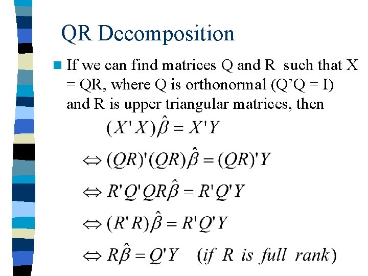
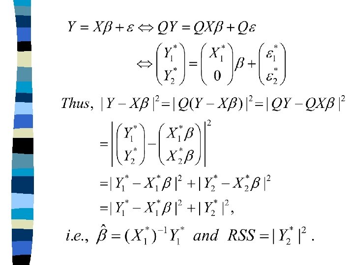
QR Decomposition n If we can find matrices Q and R such that X = QR, where Q is orthonormal (Q’Q = I) and R is upper triangular matrices, then

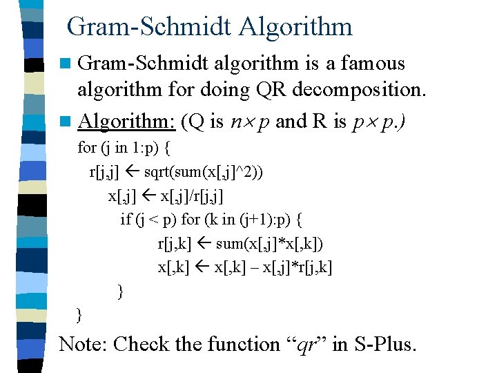
Gram-Schmidt Algorithm n Gram-Schmidt algorithm is a famous algorithm for doing QR decomposition. n Algorithm: (Q is n p and R is p p. ) for (j in 1: p) { r[j, j] sqrt(sum(x[, j]^2)) x[, j]/r[j, j] if (j < p) for (k in (j+1): p) { r[j, k] sum(x[, j]*x[, k]) x[, k] – x[, j]*r[j, k] } } Note: Check the function “qr” in S-Plus.

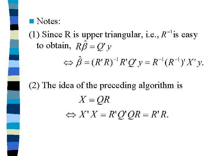
n Notes: (1) Since R is upper triangular, i. e. , to obtain, is easy (2) The idea of the preceding algorithm is

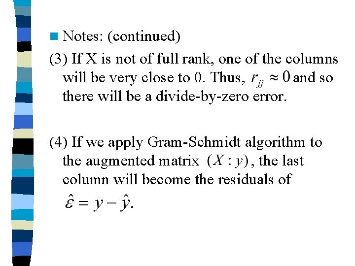
n Notes: (continued) (3) If X is not of full rank, one of the columns will be very close to 0. Thus, and so there will be a divide-by-zero error. (4) If we apply Gram-Schmidt algorithm to the augmented matrix , the last column will become the residuals of

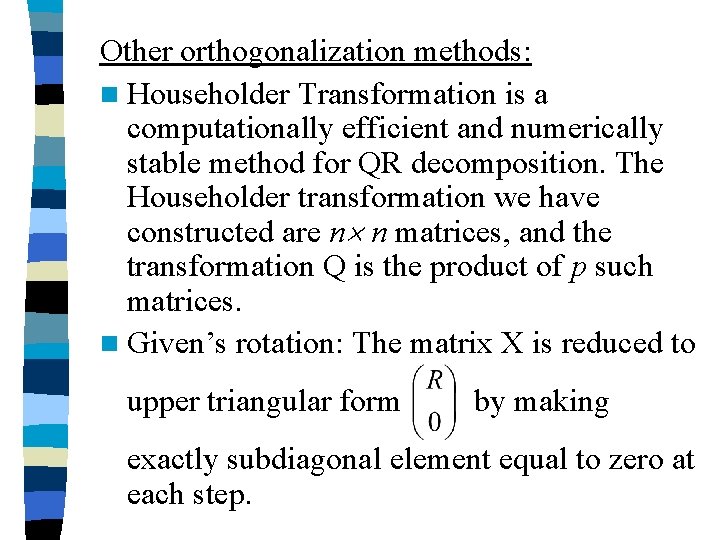
Other orthogonalization methods: n Householder Transformation is a computationally efficient and numerically stable method for QR decomposition. The Householder transformation we have constructed are n n matrices, and the transformation Q is the product of p such matrices. n Given’s rotation: The matrix X is reduced to upper triangular form by making exactly subdiagonal element equal to zero at each step.

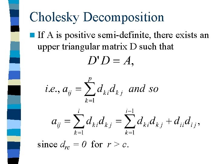
Cholesky Decomposition n If A is positive semi-definite, there exists an upper triangular matrix D such that since drc = 0 for r > c.

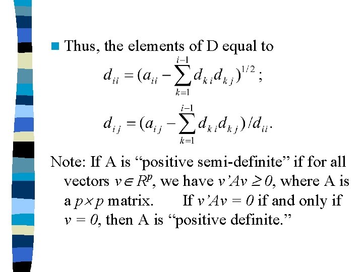
n Thus, the elements of D equal to Note: If A is “positive semi-definite” if for all vectors v Rp, we have v’Av 0, where A is a p p matrix. If v’Av = 0 if and only if v = 0, then A is “positive definite. ”

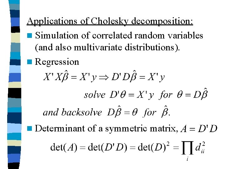
Applications of Cholesky decomposition: n Simulation of correlated random variables (and also multivariate distributions). n Regression n Determinant of a symmetric matrix,

Sweep Operator n The normal equation is not solved directly in the preceding methods. But sometimes we need to compute sums of squares and cross-products (SSCP) matrix. n This is particularly useful in stepwise regression, since we need to compute the residual sum of squares (RSS) before and after a certain variable is added or removed.

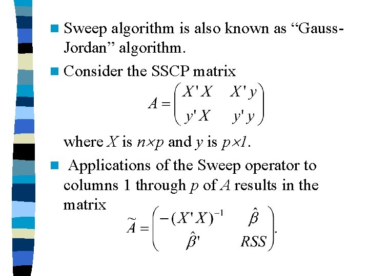
n Sweep algorithm is also known as “Gauss. Jordan” algorithm. n Consider the SSCP matrix where X is n p and y is p 1. n Applications of the Sweep operator to columns 1 through p of A results in the matrix

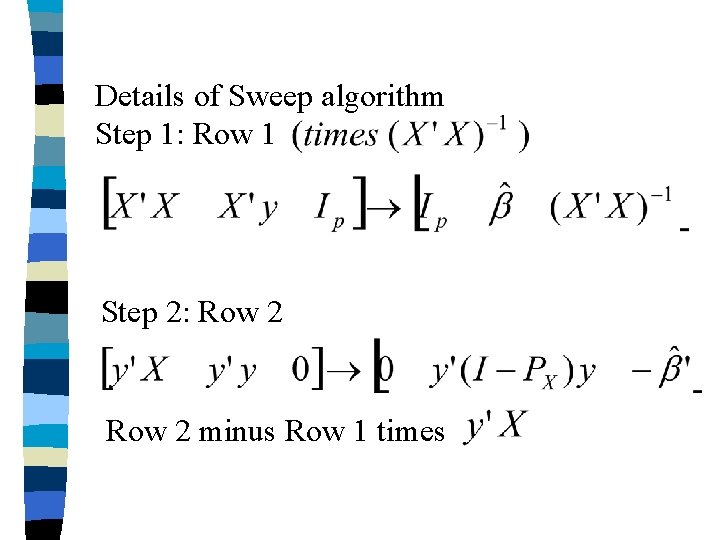
Details of Sweep algorithm Step 1: Row 1 Step 2: Row 2 minus Row 1 times

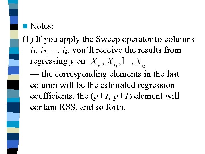
n Notes: (1) If you apply the Sweep operator to columns i 1, i 2, …, ik, you’ll receive the results from regressing y on — the corresponding elements in the last column will be the estimated regression coefficients, the (p+1, p+1) element will contain RSS, and so forth.

n Notes: (continued) (2) The Sweep operator has a simple inverse; the two together make it very easy to do stepwise regression. The SSCP matrix is symmetric, and any application of Sweep or its inverse result in a symmetric matrix, so one may take advantage of symmetric storage.

Sweep Algorithm Sweep function(A, k) { n nrow(A) for (i in (1: n)[-k]) A[i, j] – A[i, k]*A[k, j]/A[k, k] # sweep if A[k, k] > 0 # inverse if A[k, k] < 0 A[-k, k]/abs(A[k, k]) A[k, -k]/abs(A[k, k]) return(A) }

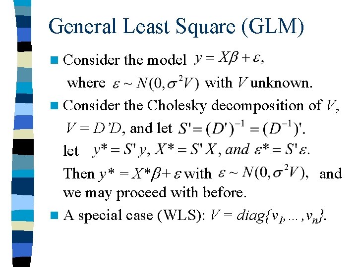
General Least Square (GLM) n Consider the model where with V unknown. n Consider the Cholesky decomposition of V, V = D’D, and let Then y* = X* + with and we may proceed with before. n A special case (WLS): V = diag{v 1, …, vn}.

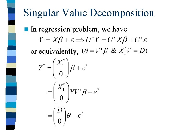
Singular Value Decomposition n In regression problem, we have or equivalently,

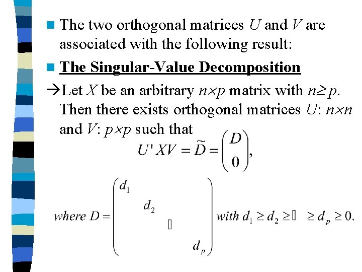
n The two orthogonal matrices U and V are associated with the following result: n The Singular-Value Decomposition Let X be an arbitrary n p matrix with n p. Then there exists orthogonal matrices U: n n and V: p p such that

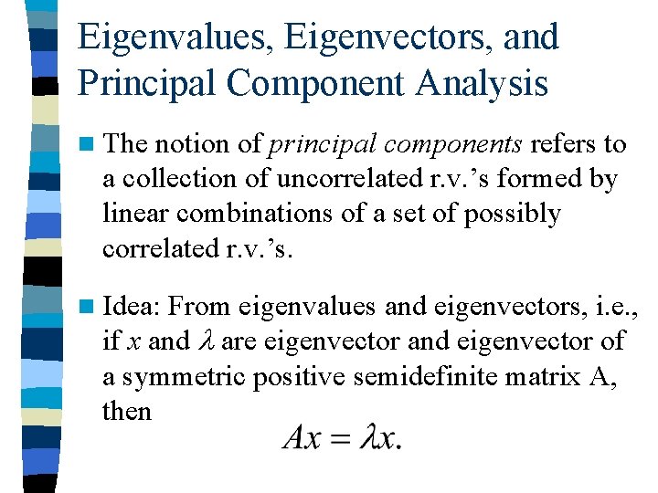
Eigenvalues, Eigenvectors, and Principal Component Analysis n The notion of principal components refers to a collection of uncorrelated r. v. ’s formed by linear combinations of a set of possibly correlated r. v. ’s. n Idea: From eigenvalues and eigenvectors, i. e. , if x and are eigenvector and eigenvector of a symmetric positive semidefinite matrix A, then

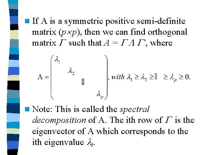
n If A is a symmetric positive semi-definite matrix (p p), then we can find orthogonal matrix such that A = ’, where n Note: This is called the spectral decomposition of A. The ith row of is the eigenvector of A which corresponds to the ith eigenvalue i.

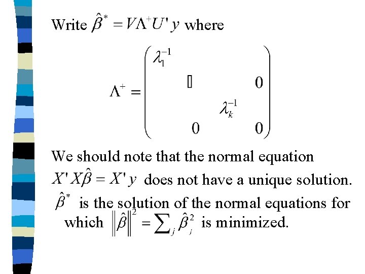
Write where We should note that the normal equation does not have a unique solution. is the solution of the normal equations for which is minimized.

Note: There are some handouts from the references regarding “Matrix Computation” n “Numerical Linear Algebra” from Internet n Chapters 3 to 6 in Monohan (2001) n Chapter 3 in Thisted (1988) Students are required to read and understand all these materials, in addition to the powerpoint notes.