Matrix balancing A matrix is unbalanced if the

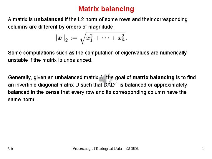
Matrix balancing A matrix is unbalanced if the L 2 norm of some rows and their corresponding columns are different by orders of magnitude. Some computations such as the computation of eigenvalues are numerically unstable if the matrix is unbalanced. Generally, given an unbalanced matrix A, the goal of matrix balancing is to find an invertible diagonal matrix D such that DAD-1 is balanced or approximately balanced in the sense that every row and its corresponding column have the same norm. V 6 Processing of Biological Data - SS 2020 1

Matrix balancing approaches Implicit matrix-balancing approaches are widely used to account for biases in Hi-C data. They rely on two different assumptions. (1) the combinatorial-bias effect between two interacting loci can be simplified as the product of the two locus-specific bias effects. (2) if there is no bias effect (that is, when all bias has been accounted for), the total genome-wide contact summation for each locus will be a constant, implying that each locus has ‘equal visibility’ to the Hi-C assay. V 6 Processing of Biological Data - SS 2020 Schmitt et al. Nature Rev Mol Cell Biol (2016) 17, 743 2

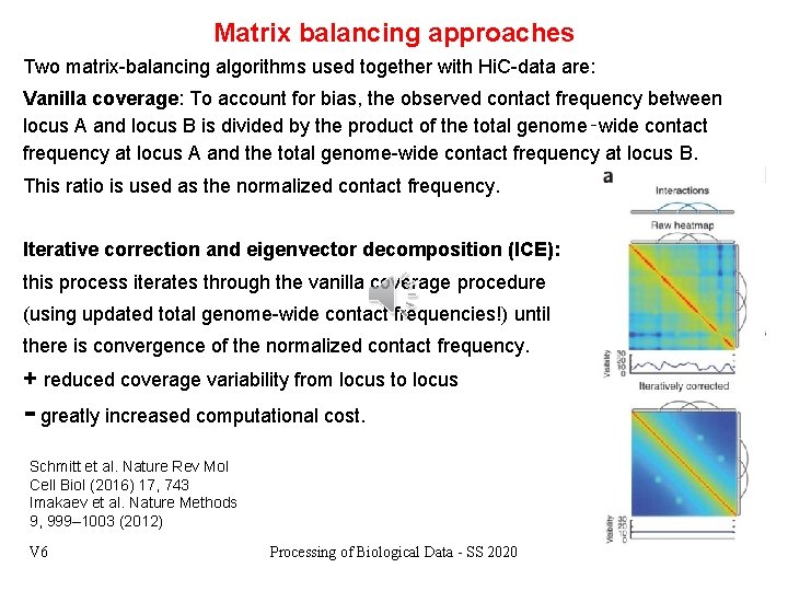
Matrix balancing approaches Two matrix-balancing algorithms used together with Hi. C-data are: Vanilla coverage: To account for bias, the observed contact frequency between locus A and locus B is divided by the product of the total genome‑wide contact frequency at locus A and the total genome-wide contact frequency at locus B. This ratio is used as the normalized contact frequency. Iterative correction and eigenvector decomposition (ICE): this process iterates through the vanilla coverage procedure (using updated total genome-wide contact frequencies!) until there is convergence of the normalized contact frequency. + reduced coverage variability from locus to locus - greatly increased computational cost. Schmitt et al. Nature Rev Mol Cell Biol (2016) 17, 743 Imakaev et al. Nature Methods 9, 999– 1003 (2012) V 6 Processing of Biological Data - SS 2020 3

Application of 4 bias removal methods: full chromosome High-resolution Hi‑C data from IMR 90 cells were processed uniformly until the bias-removal step. Then either raw contact matrices were generated (a) or normalization was conducted with one of three methods (b) to (d). Shown is data for whole human chromosome 7 for a raw Hi‑C contact matrix (part a), after normalization with Hi. CNorm (b), or with vanilla coverage (VC) (c) and iterative correction and eigenvector decomposition (ICE) (part d). V 6 Processing of Biological Data - SS 2020 Schmitt et al. Nature Rev Mol Cell Biol (2016) 17, 743 4

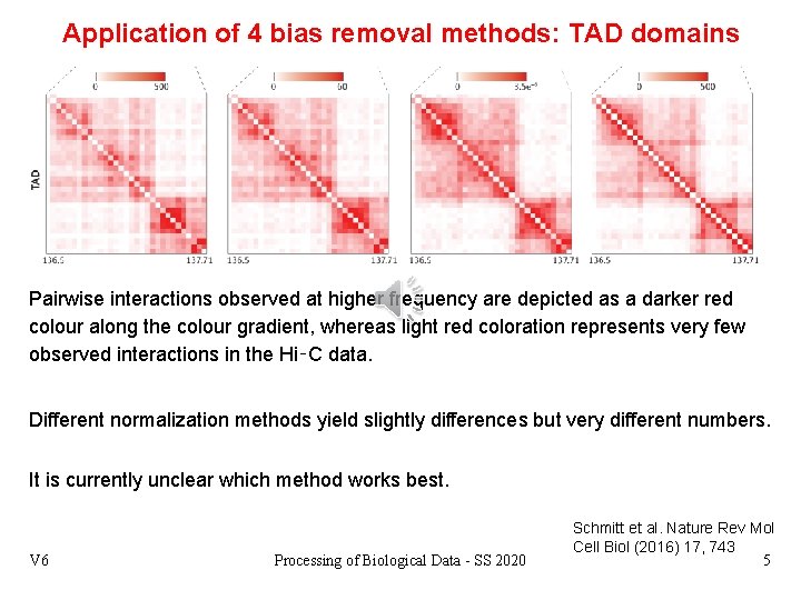
Application of 4 bias removal methods: TAD domains Pairwise interactions observed at higher frequency are depicted as a darker red colour along the colour gradient, whereas light red coloration represents very few observed interactions in the Hi‑C data. Different normalization methods yield slightly differences but very different numbers. It is currently unclear which method works best. V 6 Processing of Biological Data - SS 2020 Schmitt et al. Nature Rev Mol Cell Biol (2016) 17, 743 5

Integration of multiple data sets The group of Frank Alber/USC has originally constructed a 3 D model of the nuclear pore complex via data integration. They now work on 3 D models of chromatin. lamina-Dam. ID experiments identify specific chromatin domains with a high propensity to be located at the nuclear envelope (NE). Chromosome conformation capture experiments (Hi-C and variants) detect chromatin interactions at a genome-wide scale. V 6 Processing of Biological Data - SS 2020 Li et al. Genome Biology (2017) 18: 145 6

lamina-Dam. ID experiments Schematic illustration of DNA adenine methyltransferase identification (Dam. ID) experimental pipeline. (a) Dam only or Dam fused to a protein of interest (POI) (blue) is expressed in a suitable cell type or transgenic organism. Here: POI is lamin B 1 that is part of the nuclear lamina → DAM localizes to nuclear membrane (b) Genomic DNA is extracted. DNA obtained includes N 6‐adenine methylation sites (Me) catalyzed by Dam. (c) Genomic DNA is digested by the methylation sensitive restriction enzyme, Dpn. I. (d) Digested fragments are amplified by polymerase chain reaction (PCR). (e) Representative output indicating chromatin binding of a protein of interest at an individual locus. Vertical bars indicate the log 2 ratio of Dam‐fusion/Dam only. WIREs Dev Biol (2016) 5: 25 – 37. V 6 Processing of Biological Data - SS 2020 7

lamina-Dam. ID experiments Original Dam. ID dataset were reported by Filion et al. Here, Dam. ID was fused to 53 broadly selected chromatin proteins in Drosophila cells. PCA identified 5 chromatin types. Filion et al. Cell 143: 212 (2010) V 6 Processing of Biological Data - SS 2020 8

Integration of multiple data sets So far, most population convolution models of genome structures have typically relied on just one data type, such as Hi-C, even though a single experimental method cannot capture all aspects of the spatial genome organization. However, data are available from several technologies with complementary strengths and limitations. Integrating all these different data types should increase the accuracy and coverage of genome structure models. Moreover, such models would offer a way to cross-validate the consistency of data obtained from complementary technologies. V 6 Processing of Biological Data - SS 2020 Li et al. Genome Biology (2017) 18: 145 9

Integration of multiple data sets For example, lamina-Dam. ID experiments show a chromatin region’s probability to be close to the lamina at the nuclear envelope, whereas Hi-C experiments reveal the probability that two chromatin regions are in spatial proximity. 3 D fluorescence in situ hybridization (FISH) experiments show the distance between loci directly, and can be used to measure the distribution of distances across a population of cells. V 6 Processing of Biological Data - SS 2020 Li et al. Genome Biology (2017) 18: 145 10