MATLAB WORKSHOP Part 1 Introduction and Basics Content

MATLAB WORKSHOP Part 1: Introduction and Basics
Content • Introduction and motivation • How to work with MATLAB • Everything about variables (scalars, vectors, and matrices)
Motivation • MATLAB is widely used in industry • Solves difficult problems in a simple way.
How to work • How to get MATLAB • Work from the computer farm • Work from Technion – remote connection to the computer farm • Download the software to your PC for free through the link: http: //matlab. Technion. ac. il
Debugging • help svd • • Documentation Google Math. Works site – forum and file exchange Debugging – in the following workshops

Scalar variable For variables we use the following rules: • Names should be composed of a-z + A-Z + 0 -9 + underscore (_). • The language is Case Sensitive • Scalars can be defined in different notations:
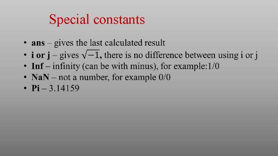
Special constants
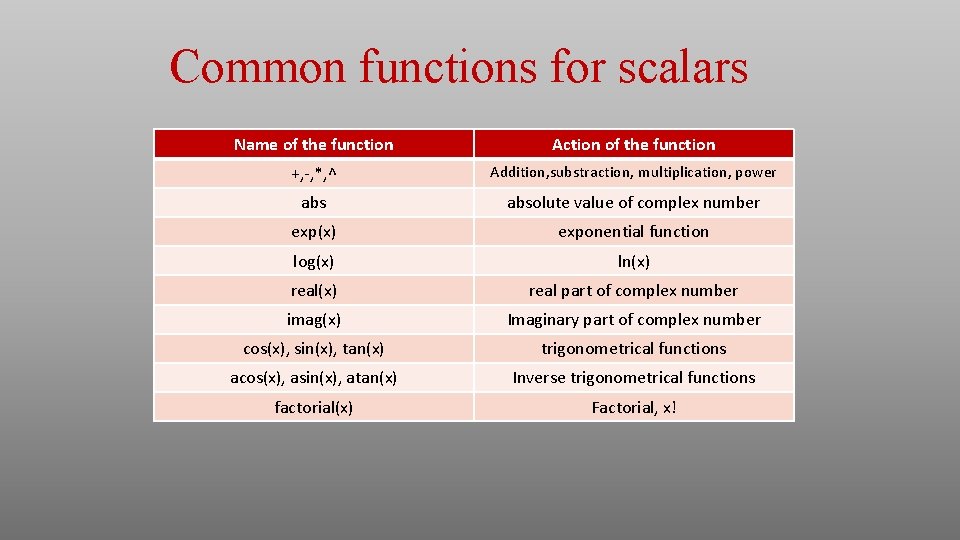
Common functions for scalars Name of the function Action of the function +, -, *, ^ Addition, substraction, multiplication, power absolute value of complex number exp(x) exponential function log(x) ln(x) real part of complex number imag(x) Imaginary part of complex number cos(x), sin(x), tan(x) trigonometrical functions acos(x), asin(x), atan(x) Inverse trigonometrical functions factorial(x) Factorial, x!
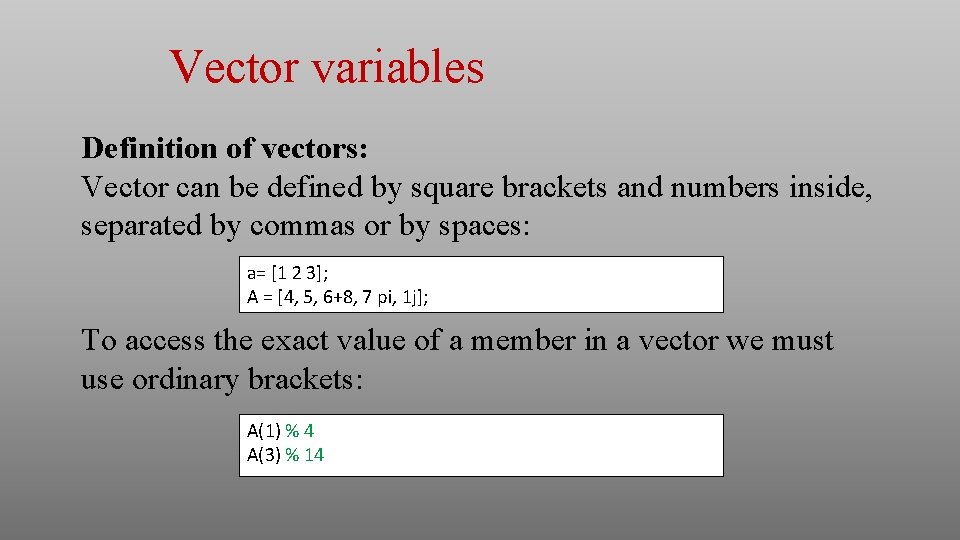
Vector variables Definition of vectors: Vector can be defined by square brackets and numbers inside, separated by commas or by spaces: a= [1 2 3]; A = [4, 5, 6+8, 7 pi, 1 j]; To access the exact value of a member in a vector we must use ordinary brackets: A(1) % 4 A(3) % 14
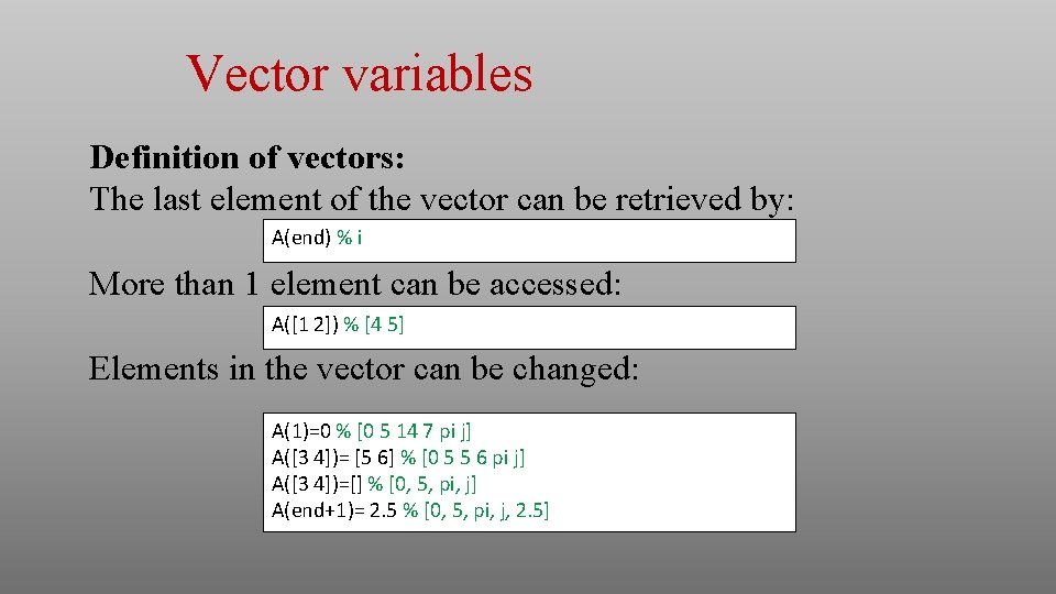
Vector variables Definition of vectors: The last element of the vector can be retrieved by: A(end) % i More than 1 element can be accessed: A([1 2]) % [4 5] Elements in the vector can be changed: A(1)=0 % [0 5 14 7 pi j] A([3 4])= [5 6] % [0 5 5 6 pi j] A([3 4])=[] % [0, 5, pi, j] A(end+1)= 2. 5 % [0, 5, pi, j, 2. 5]
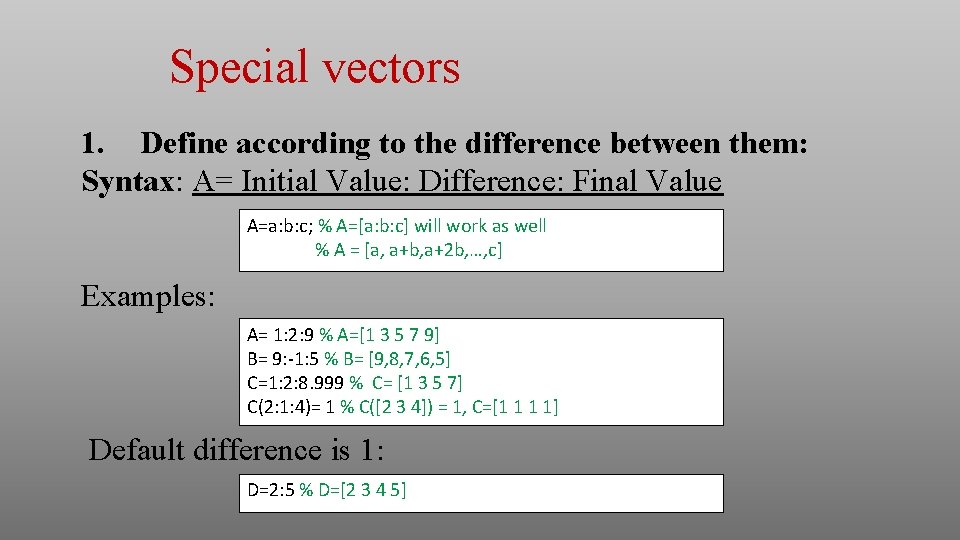
Special vectors 1. Define according to the difference between them: Syntax: A= Initial Value: Difference: Final Value A=a: b: c; % A=[a: b: c] will work as well % A = [a, a+b, a+2 b, …, c] Examples: A= 1: 2: 9 % A=[1 3 5 7 9] B= 9: -1: 5 % B= [9, 8, 7, 6, 5] C=1: 2: 8. 999 % C= [1 3 5 7] C(2: 1: 4)= 1 % C([2 3 4]) = 1, C=[1 1 1 1] Default difference is 1: D=2: 5 % D=[2 3 4 5]
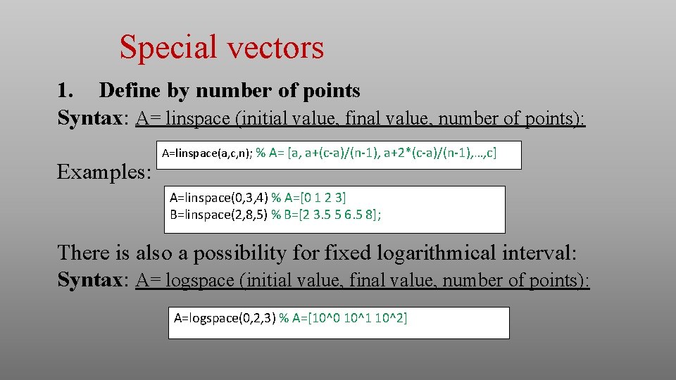
Special vectors 1. Define by number of points Syntax: A= linspace (initial value, final value, number of points): Examples: A=linspace(a, c, n); % A= [a, a+(c-a)/(n-1), a+2*(c-a)/(n-1), …, c] A=linspace(0, 3, 4) % A=[0 1 2 3] B=linspace(2, 8, 5) % B=[2 3. 5 5 6. 5 8]; There is also a possibility for fixed logarithmical interval: Syntax: A= logspace (initial value, final value, number of points): A=logspace(0, 2, 3) % A=[10^0 10^1 10^2]
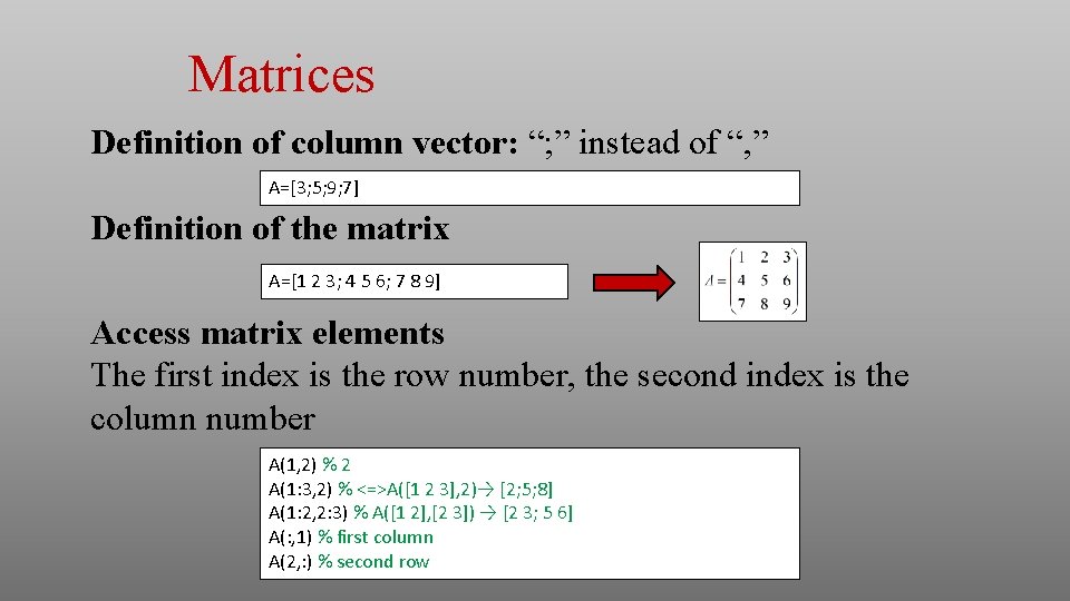
Matrices Definition of column vector: “; ” instead of “, ” A=[3; 5; 9; 7] Definition of the matrix A=[1 2 3; 4 5 6; 7 8 9] Access matrix elements The first index is the row number, the second index is the column number A(1, 2) % 2 A(1: 3, 2) % <=>A([1 2 3], 2)→ [2; 5; 8] A(1: 2, 2: 3) % A([1 2], [2 3]) → [2 3; 5 6] A(: , 1) % first column A(2, : ) % second row
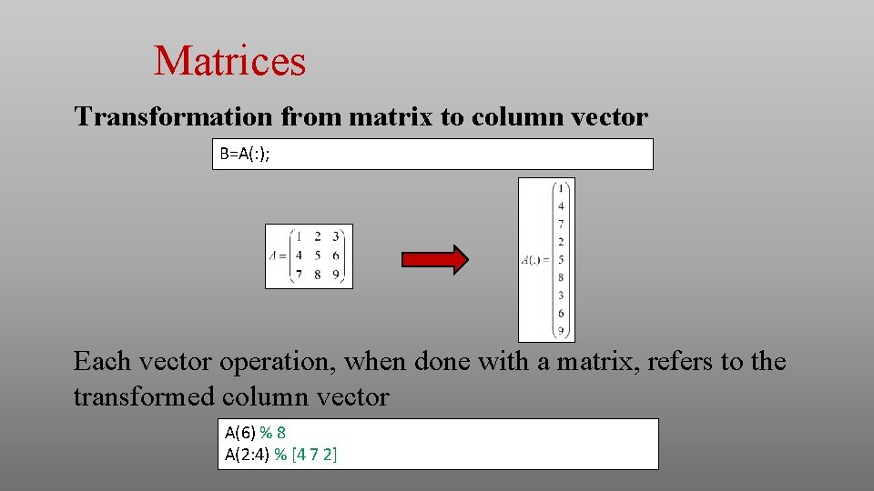
Matrices Transformation from matrix to column vector B=A(: ); Each vector operation, when done with a matrix, refers to the transformed column vector A(6) % 8 A(2: 4) % [4 7 2]
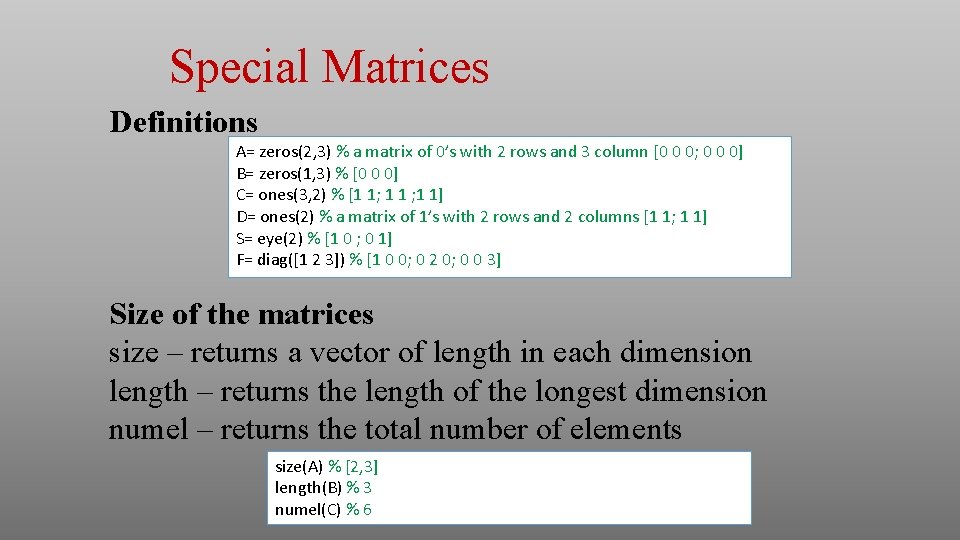
Special Matrices Definitions A= zeros(2, 3) % a matrix of 0’s with 2 rows and 3 column [0 0 0; 0 0 0] B= zeros(1, 3) % [0 0 0] C= ones(3, 2) % [1 1; 1 1] D= ones(2) % a matrix of 1’s with 2 rows and 2 columns [1 1; 1 1] S= eye(2) % [1 0 ; 0 1] F= diag([1 2 3]) % [1 0 0; 0 2 0; 0 0 3] Size of the matrices size – returns a vector of length in each dimension length – returns the length of the longest dimension numel – returns the total number of elements size(A) % [2, 3] length(B) % 3 numel(C) % 6
![Actions with vectors and matrices Operations with scalars x=[1 2 3; 5 5 0] Actions with vectors and matrices Operations with scalars x=[1 2 3; 5 5 0]](http://slidetodoc.com/presentation_image_h2/69dbf158430e4a19de7fe83df8608442/image-16.jpg)
Actions with vectors and matrices Operations with scalars x=[1 2 3; 5 5 0] y=x+2 z=x*2 Operations with matrices: + - * / - addition, subtraction, matrix multiplication, multiplication on inverse matrix. a=[1 0; 0 1]; b=[3 3; 3 3]; c=a*b
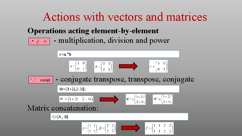
Actions with vectors and matrices Operations acting element-by-element - multiplication, division and power. *. /. ^ c=a. *b ‘. ’ conj() - conjugate transpose, conjugate W=[1+2 i, 2 -3 i]; Matrix concatenation: C=[A , B]
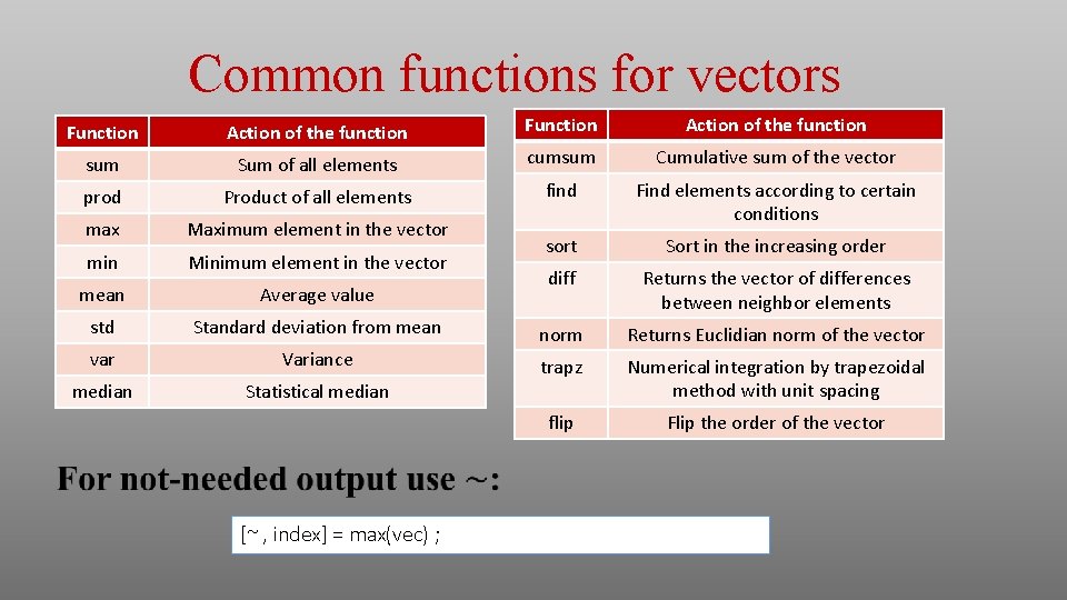
Common functions for vectors Function Action of the function sum Sum of all elements cumsum Cumulative sum of the vector prod Product of all elements find max Maximum element in the vector Find elements according to certain conditions min Minimum element in the vector sort Sort in the increasing order mean Average value diff Returns the vector of differences between neighbor elements std Standard deviation from mean norm Returns Euclidian norm of the vector var Variance trapz median Statistical median Numerical integration by trapezoidal method with unit spacing flip Flip the order of the vector [~ , index] = max(vec) ;
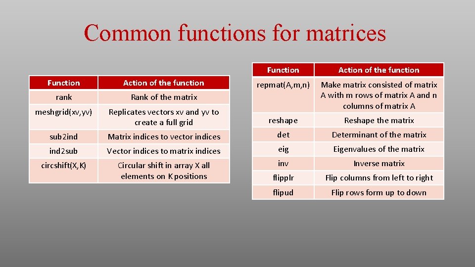
Common functions for matrices Function Action of the function repmat(A, m, n) Make matrix consisted of matrix A with m rows of matrix A and n columns of matrix A Function Action of the function rank Rank of the matrix meshgrid(xv, yv) Replicates vectors xv and yv to create a full grid reshape Reshape the matrix sub 2 ind Matrix indices to vector indices det Determinant of the matrix ind 2 sub Vector indices to matrix indices eig Eigenvalues of the matrix circshift(X, K) Circular shift in array X all elements on K positions inv Inverse matrix flipplr Flip columns from left to right flipud Flip rows form up to down
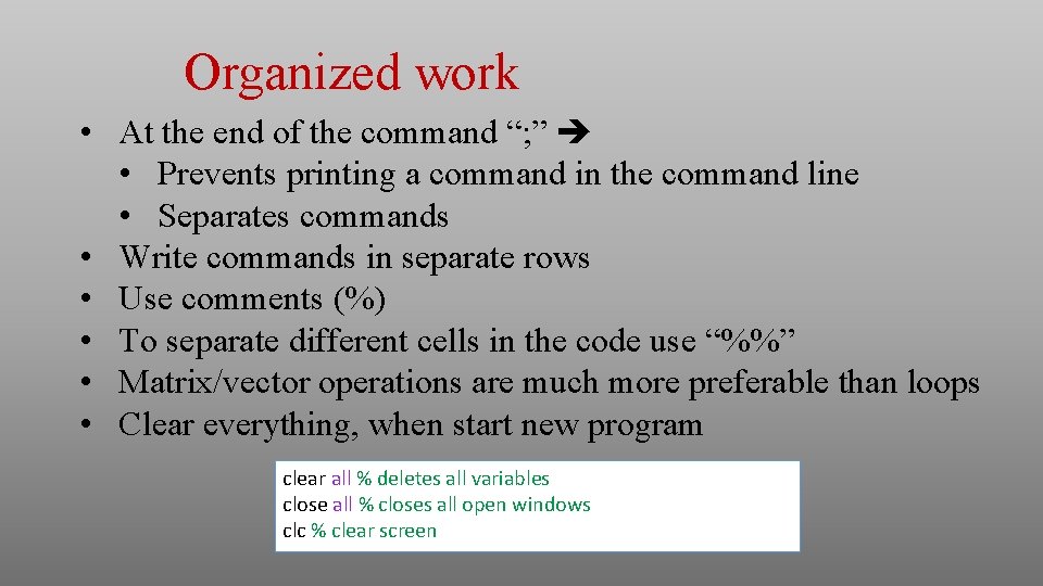
Organized work • At the end of the command “; ” • Prevents printing a command in the command line • Separates commands • Write commands in separate rows • Use comments (%) • To separate different cells in the code use “%%” • Matrix/vector operations are much more preferable than loops • Clear everything, when start new program clear all % deletes all variables close all % closes all open windows clc % clear screen
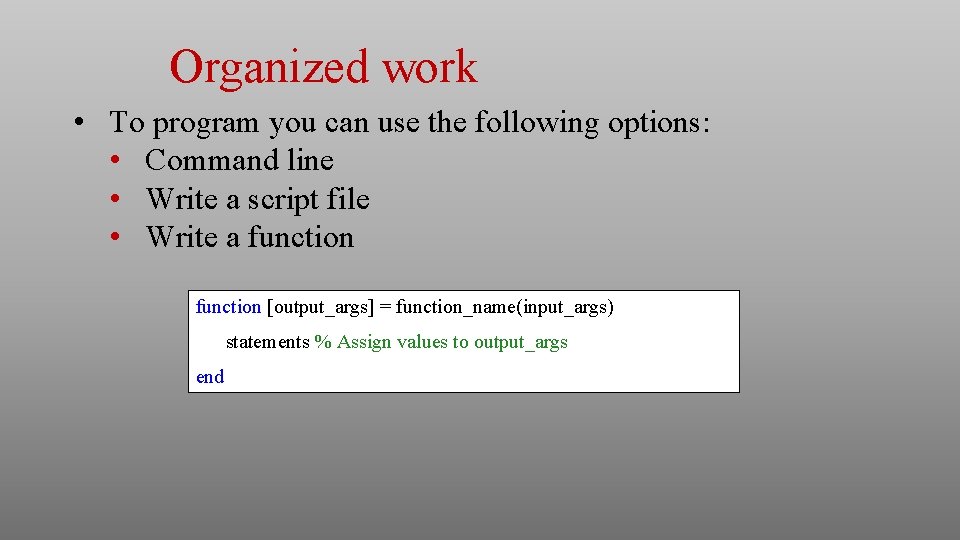
Organized work • To program you can use the following options: • Command line • Write a script file • Write a function [output_args] = function_name(input_args) statements % Assign values to output_args end
- Slides: 21