MATLAB Use of MATLAB for the courses of

MATLAB Use of MATLAB for the courses of Dinamica e Controllo dei Processi Chimici and Process Dynamics and Control Contents: PART I – Introduction elements : Polynomials and Intervals, Laplace Transforms, Partial-fractions expansion, Transfer functions PART II – Analysis of the response : Response to a step function, Response to general functions.

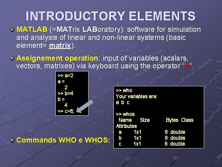
INTRODUCTORY ELEMENTS MATLAB (=MATrix LABoratory): software for simulation and analysis of linear and non-linear systems (basic element= matrix). Assignement operation: input of variables (scalars, vectors, matrixes) via keyboard using the operator “=”. >> a=2 a= 2 >> b=4 b= 4 >> c=6; Commands WHO e WHOS: >> who Your variables are: a b c >> whos Name Size Attributes a 1 x 1 b 1 x 1 c 1 x 1 Bytes Class 8 double

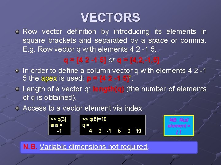
VECTORS Row vector definition by introducing its elements in square brackets and separated by a space or comma. E. g. Row vector q with elements 4 2 -1 5: q = [4 2 -1 5] or q = [4, 2, -1, 5] In order to define a column vector q with elements 4 2 -1 5 the apex is used: p = [4 2 -1 5]’. Length of a vector q: length(q) (the number of elements of q is obtained). Access to a vector element via index. >> q(3) ans = -1 >> q(6)=10 q= 4 2 -1 5 0 10 N. B. Variable dimensions not required. NB. Null element = []

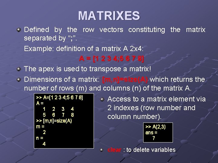
MATRIXES Defined by the row vectors constituting the matrix separated by “; ”. Example: definition of a matrix A 2 x 4: A = [1 2 3 4; 5 6 7 8] The apex is used to transpose a matrix! Dimensions of a matrix: [m, n]=size(A) which returns the number of rows (m) and columns (n) of the matrix A. >> A=[1 2 3 4; 5 6 7 8] A= 1 2 3 4 5 6 7 8 >> [m, n]=size(A) m= 2 n= 4 Access to a matrix element via 2 indexes (row number and column number). >> A(2, 3) ans = 7 clear : to delete variables

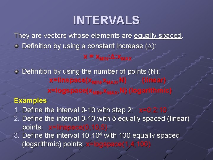
INTERVALS They are vectors whose elements are equally spaced. Definition by using a constant increase (D): x = x. MIN: D: x. MAX Definition by using the number of points (N): x=linspace(x. MIN, x. MAX, N) (linear) x=logspace(x. MIN, x. MAX, N) (logarithmic) Examples 1. Define the interval 0 -10 with step 2: x=0: 2: 10 2. Define the interval 0 -10 with 5 equally spaced (linear) points: x=linspace(0, 10, 5) 3. Define the interval 10 -104 with 100 equally spaced (logarithmic) points: x=logspace(1, 4, 100)

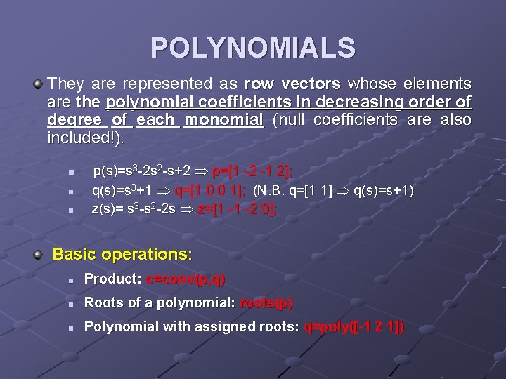
POLYNOMIALS They are represented as row vectors whose elements are the polynomial coefficients in decreasing order of degree of each monomial (null coefficients are also included!). n n n p(s)=s 3 -2 s 2 -s+2 p=[1 -2 -1 2]; q(s)=s 3+1 q=[1 0 0 1]; (N. B. q=[1 1] q(s)=s+1) z(s)= s 3 -s 2 -2 s z=[1 -1 -2 0]; Basic operations: n Product: c=conv(p, q) n Roots of a polynomial: roots(p) n Polynomial with assigned roots: q=poly([-1 2 1])

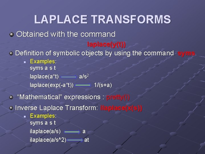
LAPLACE TRANSFORMS Obtained with the command laplace(y(t)) Definition of symbolic objects by using the command syms n Examples: syms a s t laplace(a*t) a/s 2 laplace(exp(-a*t)) 1/(s+a) “Mathematical” expressions : pretty(l) Inverse Laplace Transform: ilaplace(x(s)) n Examples: syms a s t ilaplace(a/s) ilaplace(a/s^2) a at

PARTIAL-FRACTIONS EXPANSION Obtained with the command: [c, p, k]=residue(a, b) INPUT: polynomial of the numerator (a) and polynomial of the denominator (b) of a fractional function. OUTPUT: three vectors n n n Column vector c containing the constant values Ci ; Column vector p containing the poles of the fractional function (roots of the polynomial at the denominator); Row vector k related to the direct terms (only if m>n NOT REALISTIC!!).

PARTIAL-FRACTIONS EXPANSION Example: >> a=[1 -1 -6]; >> b=[1 -2 -1 2]; >> [c, p, k]=residue(a, b) c= -1. 3333 (= -4/3) -0. 6667 (= -2/3) 3. 0000 p= 2. 0000 -1. 0000 k=

PARTIAL-FRACTIONS EXPANSION Example: Decomposition: >> a=1; >> b=poly([-2 -1 -1]) ; >> [c, p, k]=residue(a, b) c= 1. 0000 -1. 0000 p= -2. 0000 -1. 0000 k= Inverse Laplace Transforms: syms s t >> ys=1/(s+2) - 1/(s+1) + 1/(s+1)^2 ys = 1/(s+2)-1/(s+1)+1/(s+1)^2 >> pretty(ys) 1 1 1 ----- - ----- + -------s+2 s+1 2 (s + 1) >> yt=ilaplace(ys) yt = exp(-2*t)+exp(-t)*(1+t) >> pretty(yt) exp(-2 t) + exp(-t) (1 + t)

TRANSFER FUNCTIONS Polynomial assignement: G=tf(num, den) Examples: >> G=tf([1 2], [1 2 1]) Transfer function: s+2 ------s^2 + 2 s + 1 Poles of a transfer function: pole(G)

TRANSFER FUNCTIONS Assignement by zeros and poles: G=zpk(zeri, poli, gain) Example: >> zpk([3 -1], [-2 4], 5) Zero/pole/gain: 5 (s-3) (s+1) ---------(s+2) (s-4) Conversion from the “zeros-poles” to the polynomial form and vice-versa: tf(G) and zpk(G)

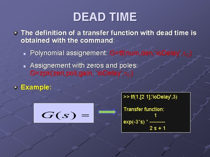
DEAD TIME The definition of a transfer function with dead time is obtained with the command: n n Polynomial assignement: G=tf(num, den, ’io. Delay’, t. D) Assignement with zeros and poles: G=zpk(zeri, poli, gain, ’io. Delay’, t. D) Example: >> tf(1, [2 1], 'io. Delay', 3) Transfer function: 1 exp(-3*s) * ----2 s+1

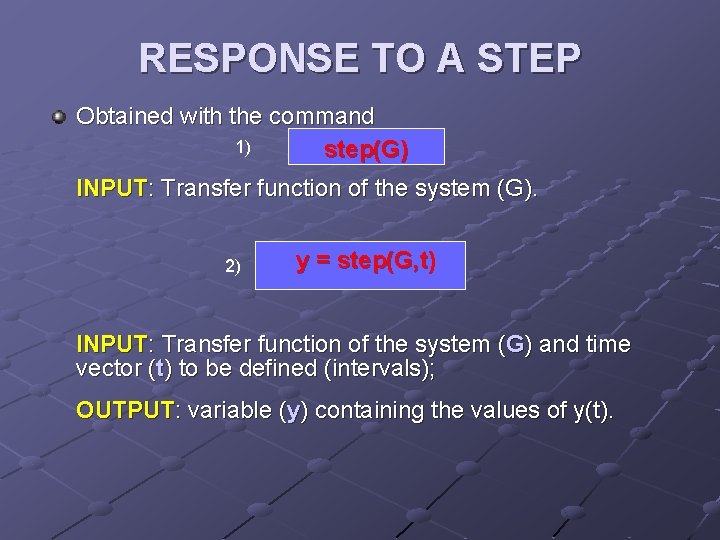
RESPONSE TO A STEP Obtained with the command 1) step(G) INPUT: Transfer function of the system (G). 2) y = step(G, t) INPUT: Transfer function of the system (G) and time vector (t) to be defined (intervals); OUTPUT: variable (y) containing the values of y(t).

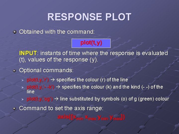
RESPONSE PLOT Obtained with the command: plot(t, y) INPUT: instants of time where the response is evaluated (t), values of the response (y). Optional commands: Ø Ø Ø plot(t, y, ’r’) specifies the colour (r) of the line plot(t, y, ’- -k’) specifies the colour (k) and the kind (- -) of the line plot(t, y, ’og’) line substituted by symbols (o) of g (green) colour Command to set the axis range: axis([xmin xmax ymin ymax])

RISPONSE TO A STEP Example: >> G=tf(1, [0. 5 1]); >> t=0: 0. 1: 10; >> y=step(G, t); >> plot(t, y, 'b') >> axis([0 4 0 1. 1]) >> xlabel('tempo [s]', 'Fontsize', 12) >> ylabel('y(t)', 'Fontsize', 12) >> title('Risposta a step', 'Fontsize', 14) >> hold

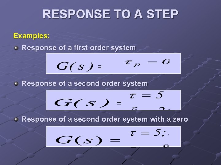
RESPONSE TO A STEP Examples: Response of a first order system Response of a second order system with a zero

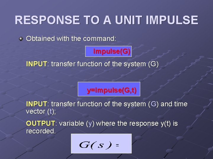
RESPONSE TO A UNIT IMPULSE Obtained with the command: impulse(G) INPUT: transfer function of the system (G) y=impulse(G, t) INPUT: transfer function of the system (G) and time vector (t); OUTPUT: variable (y) where the response y(t) is recorded.

RESPONSE TO A GENERAL FUNCTION Obtained with the command lsim(G, f) INPUT: Transfer function of the system (G) and forcing function (definition is required). y=lsim(G, f, t) INPUT: transfer function of the system (G), forcing function (definition is required) and vector of times (t); OUTPUT: variable (y) where the response y(t) is recorded.

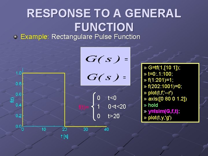
RESPONSE TO A GENERAL FUNCTION Example: Rectangulare Pulse Function f(t)= 0 1 t<0 0<t<20 0 t>20 » G=tf(1, [10 1]); » t=0: . 1: 100; » f(1: 201)=1; » f(202: 1001)=0; » plot(t, f, '--r') » axis([0 80 0 1. 2]) » hold » y=lsim(G, f, t); » plot(t, y, 'g')

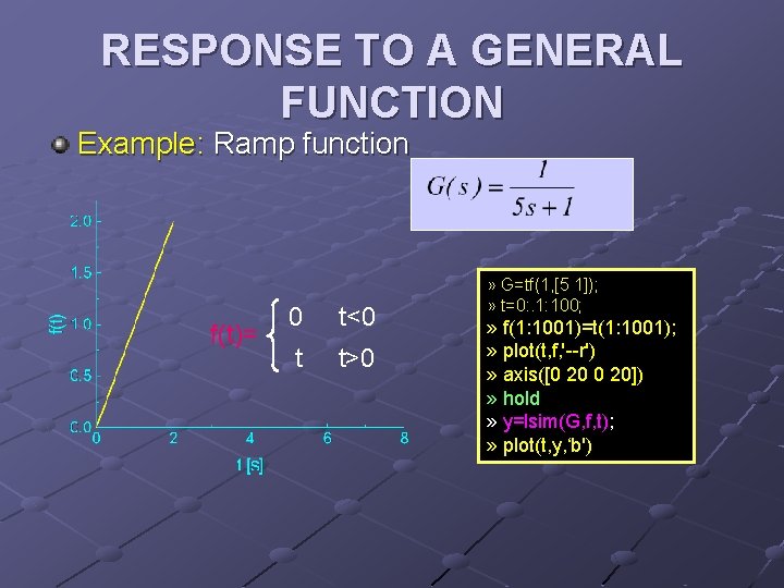
RESPONSE TO A GENERAL FUNCTION Example: Ramp function f(t)= 0 t<0 t t>0 » G=tf(1, [5 1]); » t=0: . 1: 100; » f(1: 1001)=t(1: 1001); » plot(t, f, '--r') » axis([0 20]) » hold » y=lsim(G, f, t); » plot(t, y, ‘b')

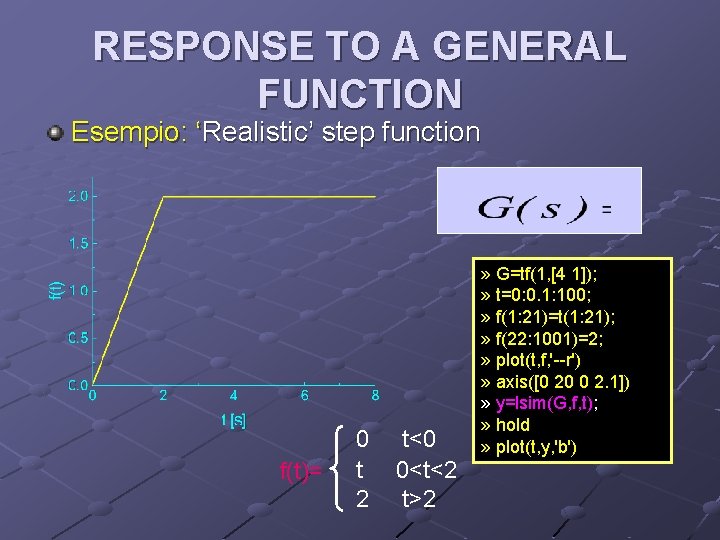
RESPONSE TO A GENERAL FUNCTION Esempio: ‘Realistic’ step function f(t)= 0 t 2 t<0 0<t<2 t>2 » G=tf(1, [4 1]); » t=0: 0. 1: 100; » f(1: 21)=t(1: 21); » f(22: 1001)=2; » plot(t, f, '--r') » axis([0 20 0 2. 1]) » y=lsim(G, f, t); » hold » plot(t, y, 'b')

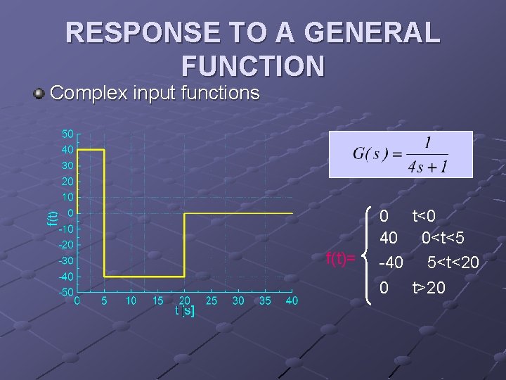
RESPONSE TO A GENERAL FUNCTION Complex input functions f(t)= 0 t<0 40 0<t<5 -40 5<t<20 0 t>20