MATLAB Tutorial Series Tuning MATLAB for Better Performance

MATLAB Tutorial Series Tuning MATLAB for Better Performance Kadin Tseng Scientific Computing and Visualization, IS&T Boston University Spring 2011 1

Topics Covered 1. Performance Issues 1. 1 Memory Allocations 1. 2 Vector Representations 1. 3 Compiler 1. 4 Other Considerations 2. Multiprocessing with MATLAB Spring 2011 2

1. Performance Issues 1. 1 Memory Access 1. 2 Vector Representations 1. 3 Compiler 1. 4 Other Considerations Spring 2011 3

1. 1 Memory Access Memory access patterns often affect computational performance. Some effective ways to enhance performance in MATLAB : § § § Allocate array memory before using it For-loops Ordering Compute and save array in-place where applicable. Spring 2011 4

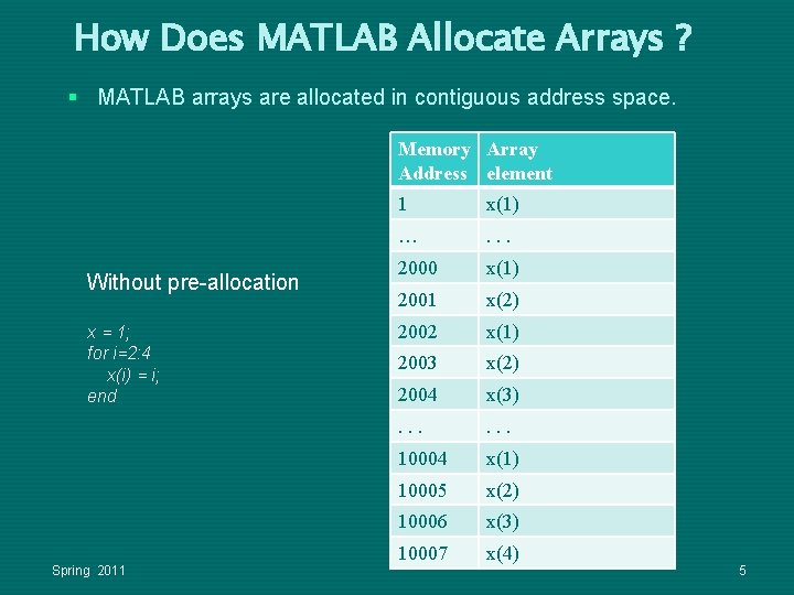
How Does MATLAB Allocate Arrays ? § MATLAB arrays are allocated in contiguous address space. Memory Array Address element Without pre-allocation x = 1; for i=2: 4 x(i) = i; end Spring 2011 1 x(1) … . . . 2000 x(1) 2001 x(2) 2002 x(1) 2003 x(2) 2004 x(3) . . . 10004 x(1) 10005 x(2) 10006 x(3) 10007 x(4) 5

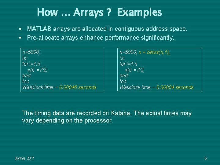
How … Arrays ? Examples § MATLAB arrays are allocated in contiguous address space. § Pre-allocate arrays enhance performance significantly. n=5000; tic for i=1: n x(i) = i^2; end toc Wallclock time = 0. 00046 seconds n=5000; x = zeros(n, 1); tic for i=1: n x(i) = i^2; end toc Wallclock time = 0. 00004 seconds The timing data are recorded on Katana. The actual times may vary depending on the processor. Spring 2011 6

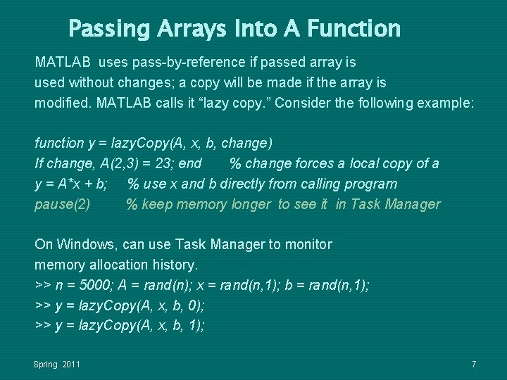
Passing Arrays Into A Function MATLAB uses pass-by-reference if passed array is used without changes; a copy will be made if the array is modified. MATLAB calls it “lazy copy. ” Consider the following example: function y = lazy. Copy(A, x, b, change) If change, A(2, 3) = 23; end % change forces a local copy of a y = A*x + b; % use x and b directly from calling program pause(2) % keep memory longer to see it in Task Manager On Windows, can use Task Manager to monitor memory allocation history. >> n = 5000; A = rand(n); x = rand(n, 1); b = rand(n, 1); >> y = lazy. Copy(A, x, b, 0); >> y = lazy. Copy(A, x, b, 1); Spring 2011 7

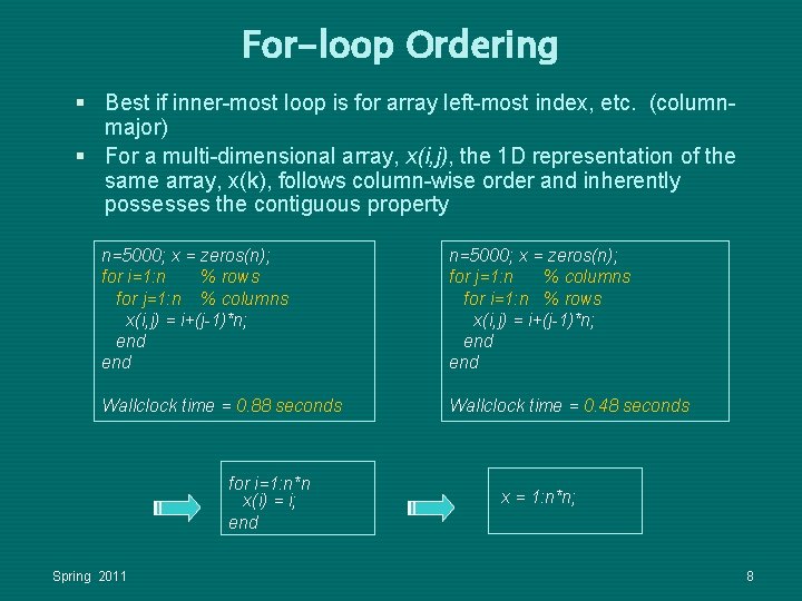
For-loop Ordering § Best if inner-most loop is for array left-most index, etc. (columnmajor) § For a multi-dimensional array, x(i, j), the 1 D representation of the same array, x(k), follows column-wise order and inherently possesses the contiguous property n=5000; x = zeros(n); for i=1: n % rows for j=1: n % columns x(i, j) = i+(j-1)*n; end n=5000; x = zeros(n); for j=1: n % columns for i=1: n % rows x(i, j) = i+(j-1)*n; end Wallclock time = 0. 88 seconds Wallclock time = 0. 48 seconds for i=1: n*n x(i) = i; end Spring 2011 x = 1: n*n; 8

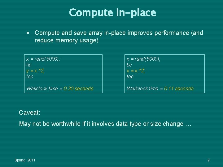
Compute In-place § Compute and save array in-place improves performance (and reduce memory usage) x = rand(5000); tic y = x. ^2; toc x = rand(5000); tic x = x. ^2; toc Wallclock time = 0. 30 seconds Wallclock time = 0. 11 seconds Caveat: May not be worthwhile if it involves data type or size change … Spring 2011 9

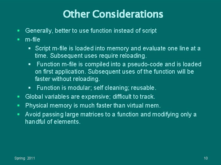
Other Considerations § Generally, better to use function instead of script § m-file § Script m-file is loaded into memory and evaluate one line at a time. Subsequent uses require reloading. § Function m-file is compiled into a pseudo-code and is loaded on first application. Subsequent uses of the function will be faster without reloading. § Function is modular; self cleaning; reusable. § Global variables are expensive; difficult to track. § Physical memory is much faster than virtual mem. § Avoid passing large matrices to a function and modifying only a handful of elements. Spring 2011 10

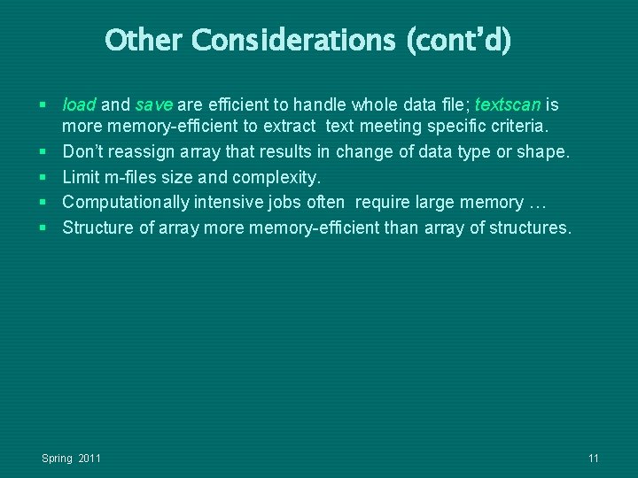
Other Considerations (cont’d) § load and save are efficient to handle whole data file; textscan is more memory-efficient to extract text meeting specific criteria. § Don’t reassign array that results in change of data type or shape. § Limit m-files size and complexity. § Computationally intensive jobs often require large memory … § Structure of array more memory-efficient than array of structures. Spring 2011 11

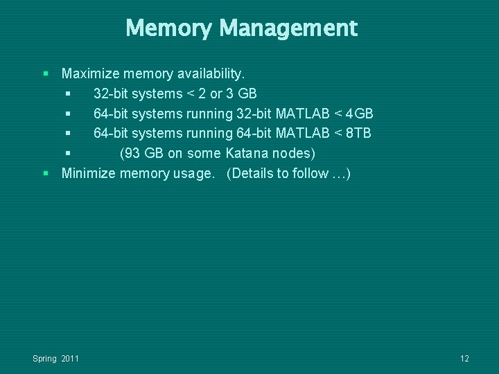
Memory Management § Maximize memory availability. § 32 -bit systems < 2 or 3 GB § 64 -bit systems running 32 -bit MATLAB < 4 GB § 64 -bit systems running 64 -bit MATLAB < 8 TB § (93 GB on some Katana nodes) § Minimize memory usage. (Details to follow …) Spring 2011 12

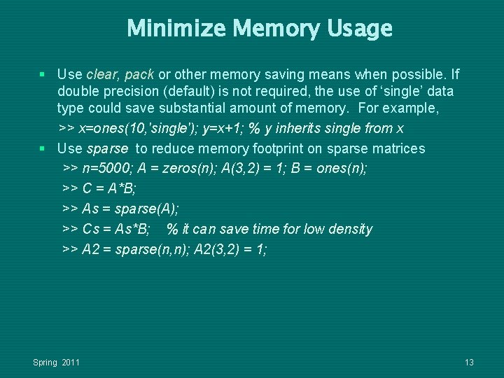
Minimize Memory Usage § Use clear, pack or other memory saving means when possible. If double precision (default) is not required, the use of ‘single’ data type could save substantial amount of memory. For example, >> x=ones(10, 'single'); y=x+1; % y inherits single from x § Use sparse to reduce memory footprint on sparse matrices >> n=5000; A = zeros(n); A(3, 2) = 1; B = ones(n); >> C = A*B; >> As = sparse(A); >> Cs = As*B; % it can save time for low density >> A 2 = sparse(n, n); A 2(3, 2) = 1; Spring 2011 13

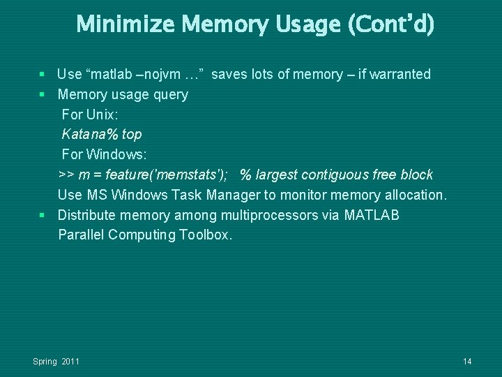
Minimize Memory Usage (Cont’d) § Use “matlab –nojvm …” saves lots of memory – if warranted § Memory usage query For Unix: Katana% top For Windows: >> m = feature('memstats'); % largest contiguous free block Use MS Windows Task Manager to monitor memory allocation. § Distribute memory among multiprocessors via MATLAB Parallel Computing Toolbox. Spring 2011 14

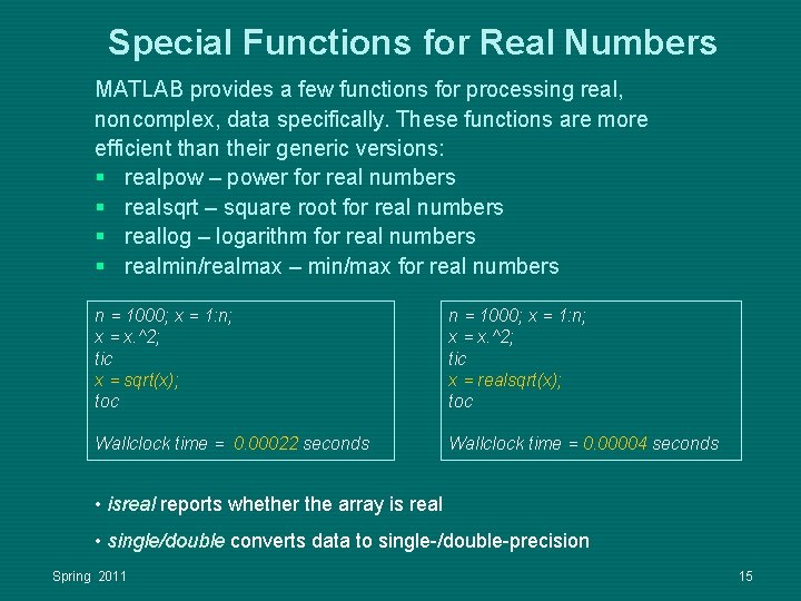
Special Functions for Real Numbers MATLAB provides a few functions for processing real, noncomplex, data specifically. These functions are more efficient than their generic versions: § realpow – power for real numbers § realsqrt – square root for real numbers § reallog – logarithm for real numbers § realmin/realmax – min/max for real numbers n = 1000; x = 1: n; x = x. ^2; tic x = sqrt(x); toc n = 1000; x = 1: n; x = x. ^2; tic x = realsqrt(x); toc Wallclock time = 0. 00022 seconds Wallclock time = 0. 00004 seconds • isreal reports whether the array is real • single/double converts data to single-/double-precision Spring 2011 15

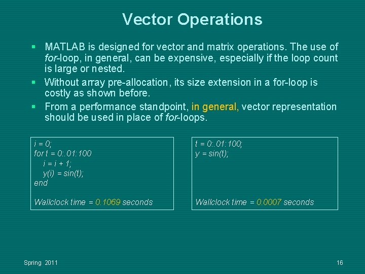
Vector Operations § MATLAB is designed for vector and matrix operations. The use of for-loop, in general, can be expensive, especially if the loop count is large or nested. § Without array pre-allocation, its size extension in a for-loop is costly as shown before. § From a performance standpoint, in general, vector representation should be used in place of for-loops. i = 0; for t = 0: . 01: 100 i = i + 1; y(i) = sin(t); end t = 0: . 01: 100; y = sin(t); Wallclock time = 0. 1069 seconds Wallclock time = 0. 0007 seconds Spring 2011 16

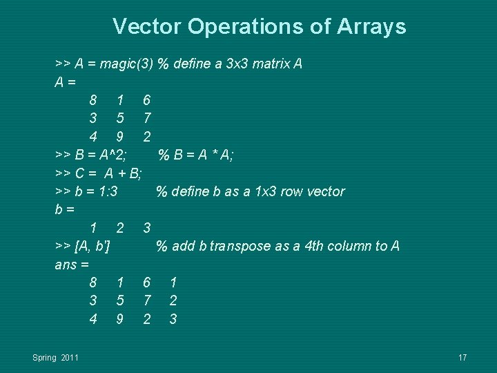
Vector Operations of Arrays >> A = magic(3) % define a 3 x 3 matrix A A= 8 1 6 3 5 7 4 9 2 >> B = A^2; % B = A * A; >> C = A + B; >> b = 1: 3 % define b as a 1 x 3 row vector b= 1 2 3 >> [A, b'] % add b transpose as a 4 th column to A ans = 8 1 6 1 3 5 7 2 4 9 2 3 Spring 2011 17

Vector Operations >> [A; b] % add b as a 4 th row to A ans = 8 1 6 3 5 7 4 9 2 1 2 3 >> A = zeros(3) % zeros generates 3*3 array of 0’s A= 0 0 0 0 0 >> B = 2*ones(2, 3) % ones generates 2 * 3 array of 1’s B= 2 2 2 Alternatively, >> B = repmat(2, 2, 3) % matrix replication Spring 2011 18

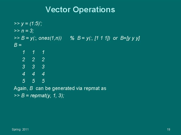
Vector Operations >> y = (1: 5)’; >> n = 3; >> B = y(: , ones(1, n)) % B = y(: , [1 1 1]) or B=[y y y] B= 1 1 1 2 2 2 3 3 3 4 4 4 5 5 5 Again, B can be generated via repmat as >> B = repmat(y, 1, 3); Spring 2011 19

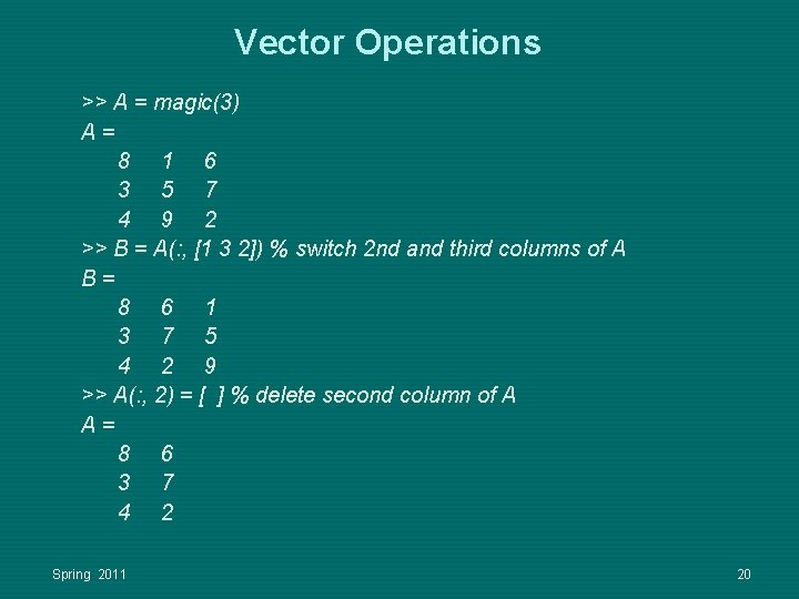
Vector Operations >> A = magic(3) A= 8 1 6 3 5 7 4 9 2 >> B = A(: , [1 3 2]) % switch 2 nd and third columns of A B= 8 6 1 3 7 5 4 2 9 >> A(: , 2) = [ ] % delete second column of A A= 8 6 3 7 4 2 Spring 2011 20

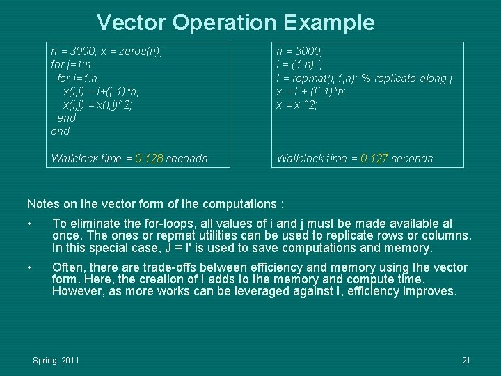
Vector Operation Example n = 3000; x = zeros(n); for j=1: n for i=1: n x(i, j) = i+(j-1)*n; x(i, j) = x(i, j)^2; end n = 3000; i = (1: n) '; I = repmat(i, 1, n); % replicate along j x = I + (I'-1)*n; x = x. ^2; Wallclock time = 0. 128 seconds Wallclock time = 0. 127 seconds Notes on the vector form of the computations : • To eliminate the for-loops, all values of i and j must be made available at once. The ones or repmat utilities can be used to replicate rows or columns. In this special case, J = I' is used to save computations and memory. • Often, there are trade-offs between efficiency and memory using the vector form. Here, the creation of I adds to the memory and compute time. However, as more works can be leveraged against I, efficiency improves. Spring 2011 21

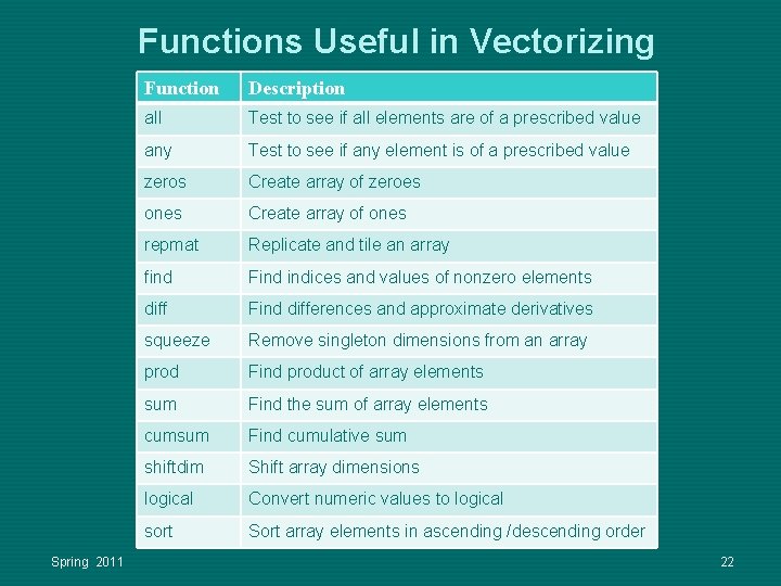
Functions Useful in Vectorizing Spring 2011 Function Description all Test to see if all elements are of a prescribed value any Test to see if any element is of a prescribed value zeros Create array of zeroes ones Create array of ones repmat Replicate and tile an array find Find indices and values of nonzero elements diff Find differences and approximate derivatives squeeze Remove singleton dimensions from an array prod Find product of array elements sum Find the sum of array elements cumsum Find cumulative sum shiftdim Shift array dimensions logical Convert numeric values to logical sort Sort array elements in ascending /descending order 22

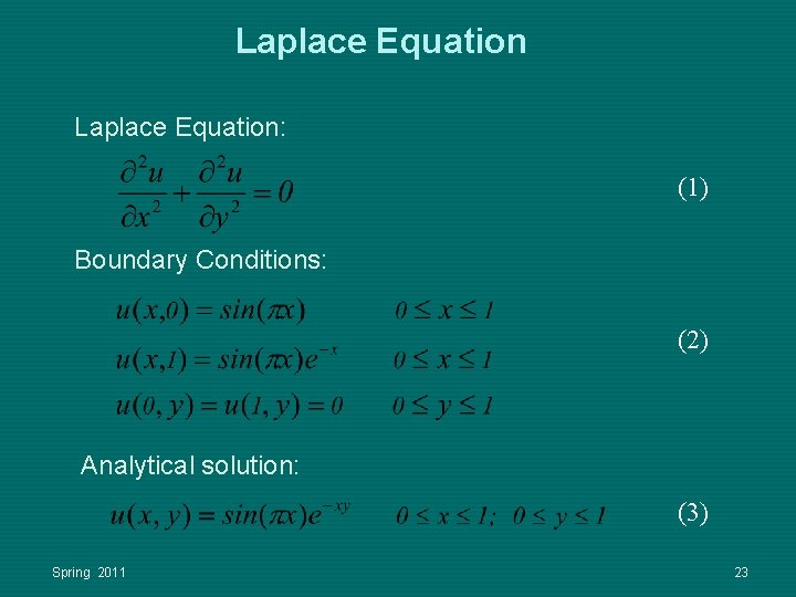
Laplace Equation: (1) Boundary Conditions: (2) Analytical solution: (3) Spring 2011 23

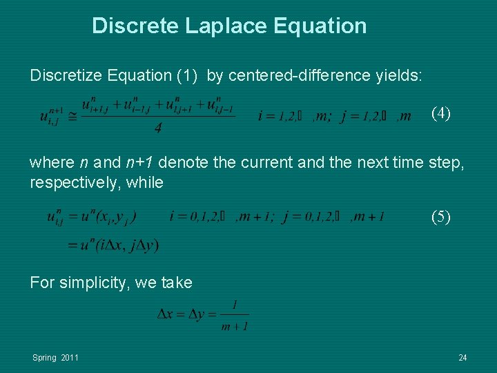
Discrete Laplace Equation Discretize Equation (1) by centered-difference yields: (4) where n and n+1 denote the current and the next time step, respectively, while (5) For simplicity, we take Spring 2011 24

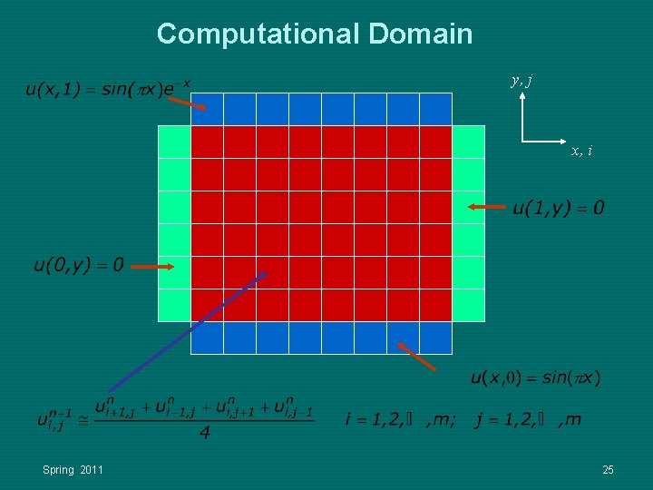
Computational Domain y, j x, i Spring 2011 25

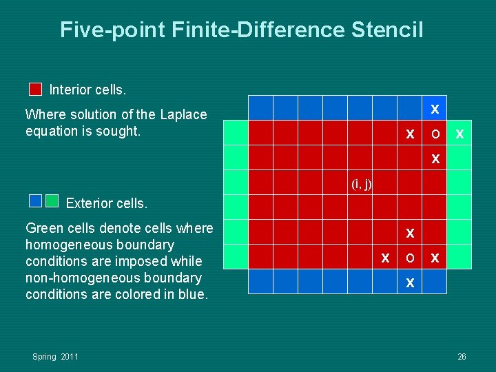
Five-point Finite-Difference Stencil Interior cells. x x o x x Where solution of the Laplace equation is sought. (i, j) Exterior cells. Green cells denote cells where homogeneous boundary conditions are imposed while non-homogeneous boundary conditions are colored in blue. Spring 2011 x x o x x 26

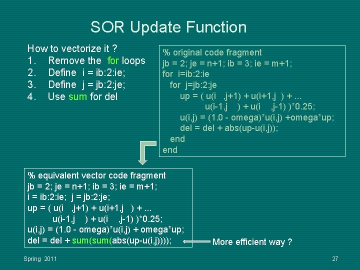
SOR Update Function How to vectorize it ? 1. Remove the for loops 2. Define i = ib: 2: ie; 3. Define j = jb: 2: je; 4. Use sum for del % original code fragment jb = 2; je = n+1; ib = 3; ie = m+1; for i=ib: 2: ie for j=jb: 2: je up = ( u(i , j+1) + u(i+1, j ) +. . . u(i-1, j ) + u(i , j-1) )*0. 25; u(i, j) = (1. 0 - omega)*u(i, j) +omega*up; del = del + abs(up-u(i, j)); end % equivalent vector code fragment jb = 2; je = n+1; ib = 3; ie = m+1; i = ib: 2: ie; j = jb: 2: je; up = ( u(i , j+1) + u(i+1, j ) +. . . u(i-1, j ) + u(i , j-1) )*0. 25; u(i, j) = (1. 0 - omega)*u(i, j) + omega*up; del = del + sum(abs(up-u(i, j)))); Spring 2011 More efficient way ? 27

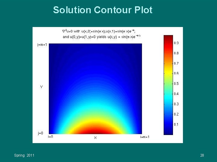
Solution Contour Plot Spring 2011 28

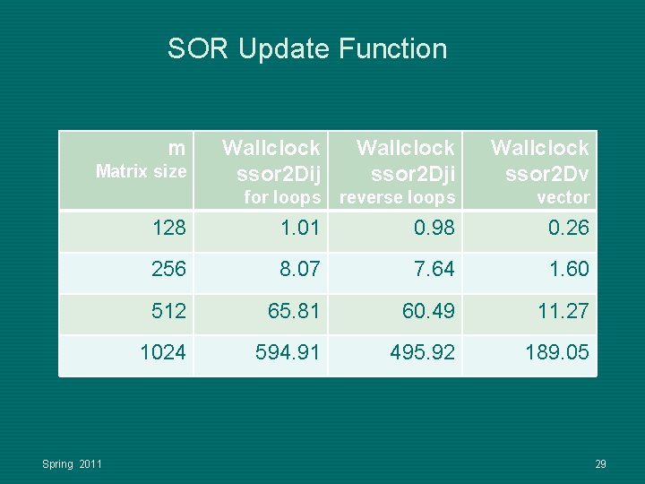
SOR Update Function m Wallclock ssor 2 Dij Wallclock ssor 2 Dji Wallclock ssor 2 Dv for loops reverse loops vector 128 1. 01 0. 98 0. 26 256 8. 07 7. 64 1. 60 512 65. 81 60. 49 11. 27 1024 594. 91 495. 92 189. 05 Matrix size Spring 2011 29

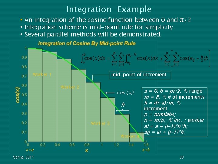
Integration Example • An integration of the cosine function between 0 and • Integration scheme is mid-point rule for simplicity. • Several parallel methods will be demonstrated. mid-point of increment Worker 1 Worker 2 cos(x) h Worker 3 Worker 4 x=a Spring 2011 π/2 a = 0; b = pi/2; % range m = 8; % # of increments h = (b-a)/m; % increment p = numlabs; n = m/p; % inc. / worker ai = a + (i-1)*n*h; aij = ai + (j-1)*h; x=b 30

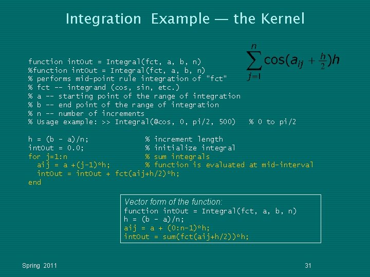
Integration Example — the Kernel function int. Out = Integral(fct, a, b, n) % performs mid-point rule integration of "fct" % fct -- integrand (cos, sin, etc. ) % a -- starting point of the range of integration % b –- end point of the range of integration % n -- number of increments % Usage example: >> Integral(@cos, 0, pi/2, 500) % 0 to pi/2 h = (b – a)/n; % increment length int. Out = 0. 0; % initialize integral for j=1: n % sum integrals aij = a +(j-1)*h; % function is evaluated at mid-interval int. Out = int. Out + fct(aij+h/2)*h; end Vector form of the function: function int. Out = Integral(fct, a, b, n) h = (b – a)/n; aij = a + (0: n-1)*h; int. Out = sum(fct(aij+h/2))*h; Spring 2011 31

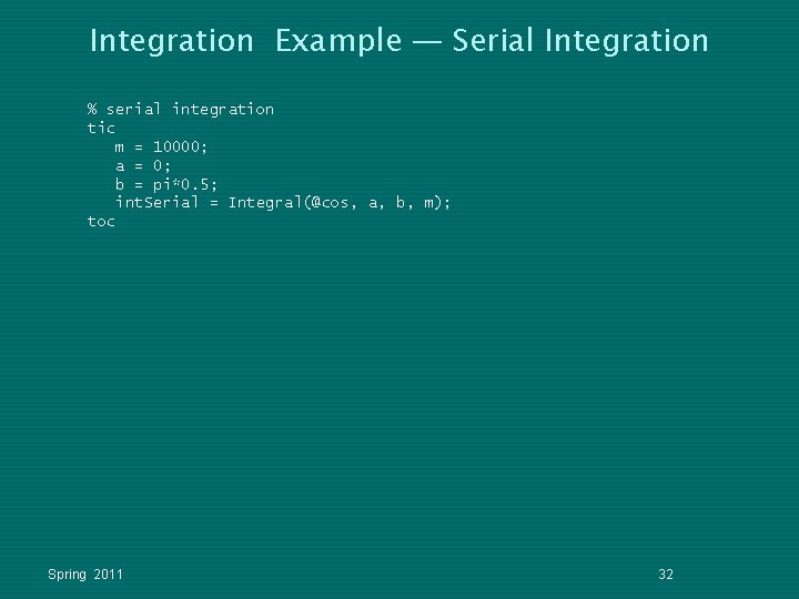
Integration Example — Serial Integration % serial integration tic m = 10000; a = 0; b = pi*0. 5; int. Serial = Integral(@cos, a, b, m); toc Spring 2011 32

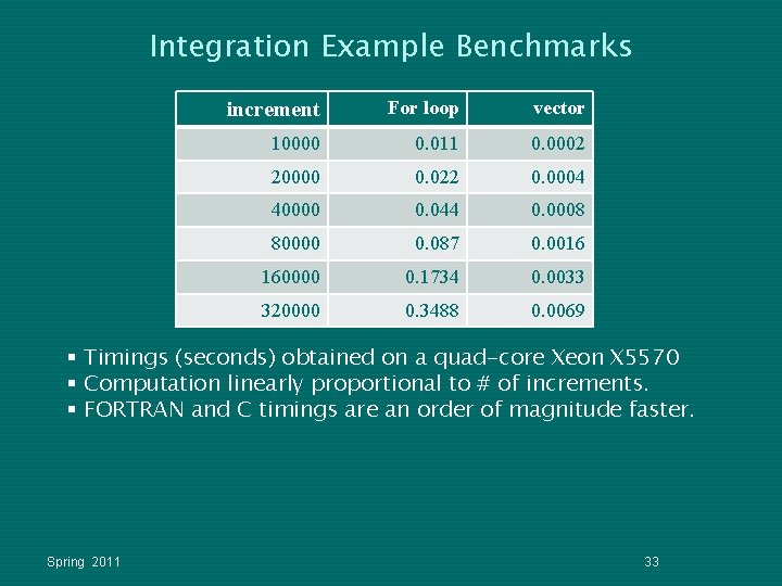
Integration Example Benchmarks increment For loop vector 10000 0. 011 0. 0002 20000 0. 022 0. 0004 40000 0. 044 0. 0008 80000 0. 087 0. 0016 160000 0. 1734 0. 0033 320000 0. 3488 0. 0069 § Timings (seconds) obtained on a quad-core Xeon X 5570 § Computation linearly proportional to # of increments. § FORTRAN and C timings are an order of magnitude faster. Spring 2011 33

Compiler mcc is a MATLAB compiler: § It compiles m-files into C codes, object libraries, or stand-alone executables. § A stand-alone executable generated with mcc can run on compatible platforms without an installed MATLAB or a MATLAB license. § Many MATLAB general and toolbox licenses are available. Infrequently, MATLAB access may be denied if all licenses are checked out. Running a stand-alone requires NO licenses and no waiting. Spring 2011 34

Compiler (Cont’d) § Some compiled codes may run more efficiently than m-files because they are not run in interpretive mode. § A stand-alone enables you to share it without revealing the source. www. bu. edu/tech/research/training/tutorials/matlab/vector/miscs/compiler/ Spring 2011 35

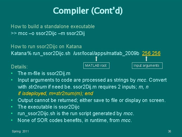
Compiler (Cont’d) How to build a standalone executable >> mcc –o ssor 2 Dijc –m ssor 2 Dij How to run ssor 2 Dijc on Katana% run_ssor 2 Dijc. sh /usr/local/apps/matlab_2009 b 256 Input arguments MATLAB root Details: • The m-file is ssor 2 Dij. m • Input arguments to code are processed as strings by mcc. Convert with str 2 num if need be. ssor 2 Dij. m requires 2 inputs; m, n if isdeployed, m=str 2 num(m); end • Output cannot be returned; either save to file or display on screen. • The executable is ssor 2 Dijc • run_ssor 2 Dijc. sh is the run script generated by mcc. • None of SOR codes benefits, in runtime, from mcc. Spring 2011 36

MATLAB Programming Tools § profile - profiler to identify “hot spots” for performance enhancement. § mlint - for inconsistencies and suspicious constructs in M-files. § debug - MATLAB debugger. § guide - Graphical User Interface design tool. Spring 2011 37

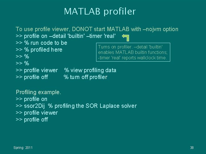
MATLAB profiler To use profile viewer, DONOT start MATLAB with –nojvm option >> profile on –detail 'builtin' –timer 'real' >> % run code to be Turns on profiler. –detail 'builtin' >> % profiled here enables MATLAB builtin functions; >> % -timer 'real' reports wallclock time. >> % >> profile viewer % view profiling data >> profile off % turn off profiler Profiling example. >> profile on >> ssor 2 Dij % profiling the SOR Laplace solver >> profile viewer >> profile off Spring 2011 38

How to Save Profiling Data Two ways to save profiling data: 1. Save into a directory of HTML files Viewing is static, i. e. , the profiling data displayed correspond to a prescribed set of options. View with a browser. 2. Saved as a MAT file Viewing is dynamic; you can change the options. Must be viewed in the MATLAB environment. Spring 2011 39

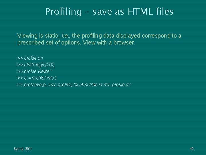
Profiling – save as HTML files Viewing is static, i. e. , the profiling data displayed correspond to a prescribed set of options. View with a browser. >> profile on >> plot(magic(20)) >> profile viewer >> p = profile('info'); >> profsave(p, ‘my_profile') % html files in my_profile dir Spring 2011 40

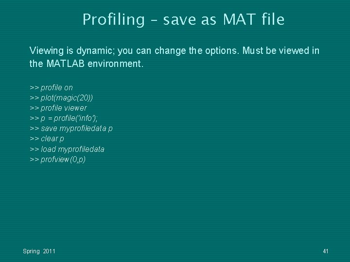
Profiling – save as MAT file Viewing is dynamic; you can change the options. Must be viewed in the MATLAB environment. >> profile on >> plot(magic(20)) >> profile viewer >> p = profile('info'); >> save myprofiledata p >> clear p >> load myprofiledata >> profview(0, p) Spring 2011 41

MATLAB “grammar checker” § mlint is used to identify coding inconsistencies and make coding performance improvement recommendations. § mlint is a standalone utility; it is an option in profile. § MATLAB editor provides this feature. § Debug mode can also be invoked through editor. Spring 2011 42

Running MATLAB in Command Line Mode and Batch Katana% matlab -nodisplay –nosplash –r “n=4, myfile(n); exit” Add –nojvm to save memory if Java is not required For batch jobs on Katana, use the above command in the batch script. Visit http: //www. bu. edu/tech/research/computation/linuxcluster/katana-cluster/runningjobs/ for instructions on running batch jobs. Spring 2011 43

Comment Out Block Of Statements On occasions, one wants to comment out an entire block of lines. If you use the MATLAB editor: • Select statement block with mouse, then – press Ctrl R keys to insert % to column 1 of each line. – press Ctrl T keys to remove % on column 1 of each line. If you use another editor: • %{ n = 3000; x = rand(n); %} • if 0 n = 3000; x = rand(n); end Spring 2011

Multiprocessing With MATLAB • Explicit parallel operations MATLAB Parallel Computing Toolbox Tutorial www. bu. edu/tech/research/training/tutorials/matlab-pct/ • Implicit parallel operations – Require shared-memory computer architecture (i. e. , multicore). – Feature on by default. Turn it off with katana% matlab –single. Comp. Thread – Specify number of threads with max. Num. Comp. Threads To be deprecated. Still supported on Version 2010 b – Activated by vector operation of applications such as hyperbolic or trigonometric functions, some La. PACK routines, Level-3 BLAS. – See “Implicit Parallelism” section of the above link. Spring 2011 45

Useful SCV Info Please help us do better in the future by participating in a quick survey: http: //scv. bu. edu/survey/spring 11 tut_survey. html § SCV home page (http: //scv. bu. edu/) § Resource Applications (https: //acct. bu. edu/SCF) § Help § Web-based tutorials (http: //scv. bu. edu/) § (MPI, Open. MP, MATLAB, IDL, Graphics tools) § HPC consultations by appointment § Kadin Tseng (kadin@bu. edu) § Doug Sondak (sondak@bu. edu) § help@twister. bu. edu, help@katana. bu. edu Spring 2011 46