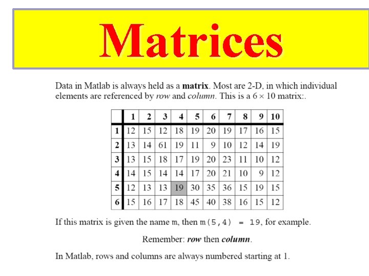
Matlab Tutorial Matrices Matrices Matrices Rows and columns

Matlab Tutorial
Matrices
Matrices
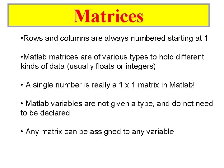
Matrices • Rows and columns are always numbered starting at 1 • Matlab matrices are of various types to hold different kinds of data (usually floats or integers) • A single number is really a 1 x 1 matrix in Matlab! • Matlab variables are not given a type, and do not need to be declared • Any matrix can be assigned to any variable
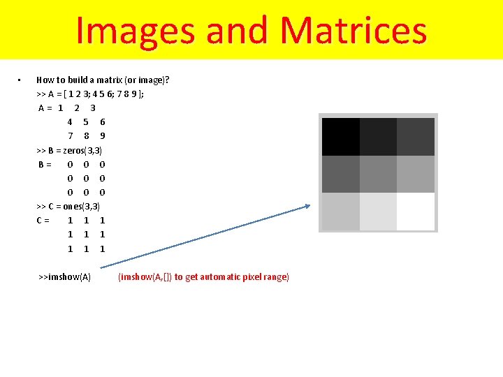
Images and Matrices How to build a matrix (or image)? >> A = [ 1 2 3; 4 5 6; 7 8 9 ]; A = 1 2 3 4 5 6 7 8 9 >> B = zeros(3, 3) B = 0 0 0 0 0 >> C = ones(3, 3) C = 1 1 1 1 1 • >>imshow(A) (imshow(A, []) to get automatic pixel range)
![Building Matrices Building matrices with [ ]: A = [2 7 4] 2 7 Building Matrices Building matrices with [ ]: A = [2 7 4] 2 7](http://slidetodoc.com/presentation_image_h/229b9dfed465816a40d1835bd514126f/image-6.jpg)
Building Matrices Building matrices with [ ]: A = [2 7 4] 2 7 4 A = [2; 7; 4] 2 7 4 A = [2 7 4; 3 8 9] 2 7 4 3 8 9 B = [ A A ] 2? 7 4 2 7 4 3 8 9
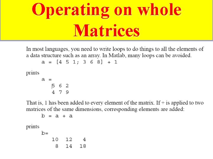
Operating on whole Matrices
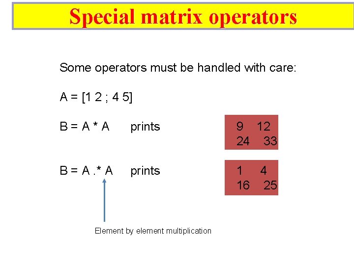
Special matrix operators Some operators must be handled with care: A = [1 2 ; 4 5] B = A * A prints B = A. * A prints Element by element multiplication 9 12 24 33 1 4 16 25
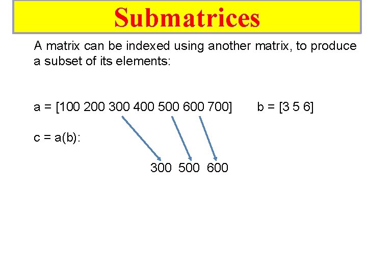
Submatrices A matrix can be indexed using another matrix, to produce a subset of its elements: a = [100 200 300 400 500 600 700] b = [3 5 6] c = a(b): 300 500 600
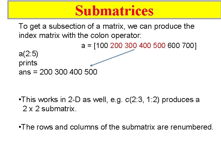
Submatrices To get a subsection of a matrix, we can produce the index matrix with the colon operator: a = [100 200 300 400 500 600 700] a(2: 5) prints ans = 200 300 400 500 • This works in 2 -D as well, e. g. c(2: 3, 1: 2) produces a 2 x 2 submatrix. • The rows and columns of the submatrix are renumbered.
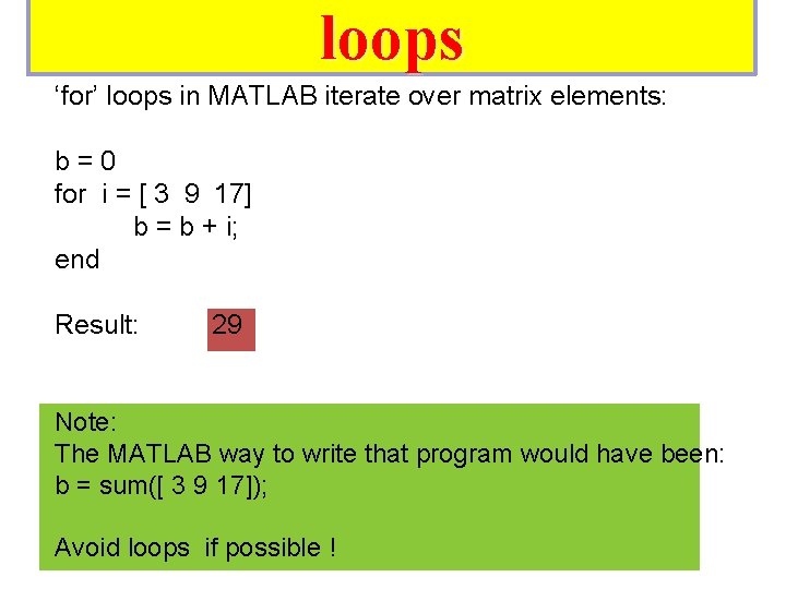
loops ‘for’ loops in MATLAB iterate over matrix elements: b = 0 for i = [ 3 9 17] b = b + i; end Result: 29 Note: The MATLAB way to write that program would have been: b = sum([ 3 9 17]); Avoid loops if possible !
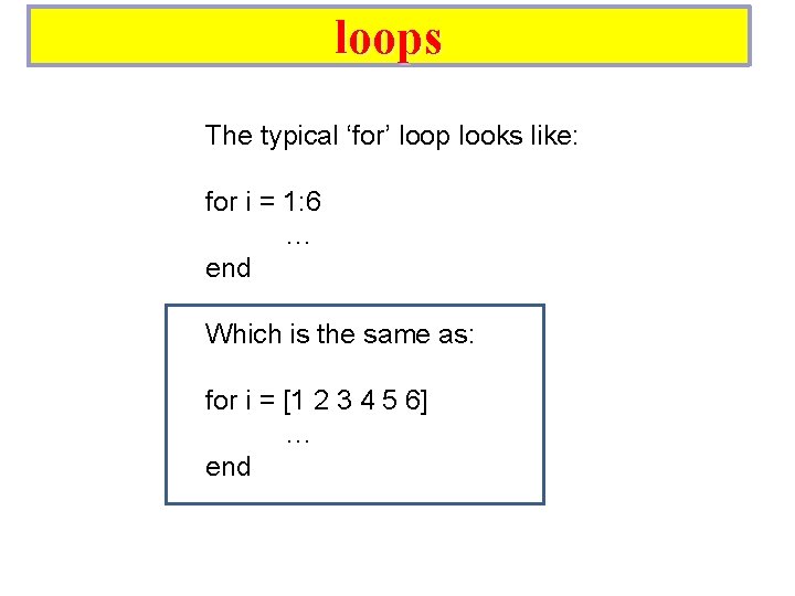
loops The typical ‘for’ loop looks like: for i = 1: 6 … end Which is the same as: for i = [1 2 3 4 5 6] … end
![Famous Matrix Manipulation Algorithms • Singular value decomposition---[U, S, V]=svd(A) • Eigenvalues and eigenvectors---[V, Famous Matrix Manipulation Algorithms • Singular value decomposition---[U, S, V]=svd(A) • Eigenvalues and eigenvectors---[V,](http://slidetodoc.com/presentation_image_h/229b9dfed465816a40d1835bd514126f/image-13.jpg)
Famous Matrix Manipulation Algorithms • Singular value decomposition---[U, S, V]=svd(A) • Eigenvalues and eigenvectors---[V, D] = eig(A) • Orthogonal-triangular decomposition- [Q, R]=qr(A) • LU factorization --[L, U] = lu(A) • Matrix rank -- a=rank(A) • Condition number -- a=cond(A) Linear systems: Ab solves A*x = b
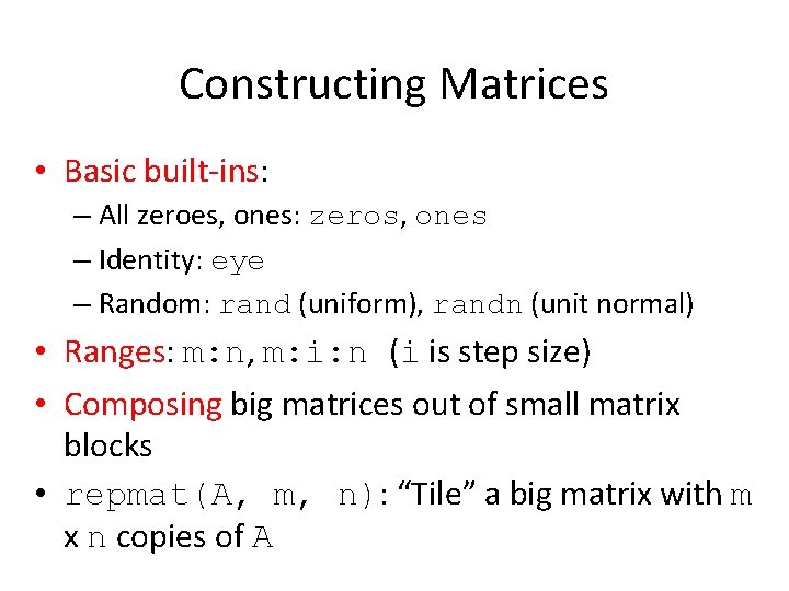
Constructing Matrices • Basic built-ins: – All zeroes, ones: zeros, ones – Identity: eye – Random: rand (uniform), randn (unit normal) • Ranges: m: n, m: i: n (i is step size) • Composing big matrices out of small matrix blocks • repmat(A, m, n): “Tile” a big matrix with m x n copies of A
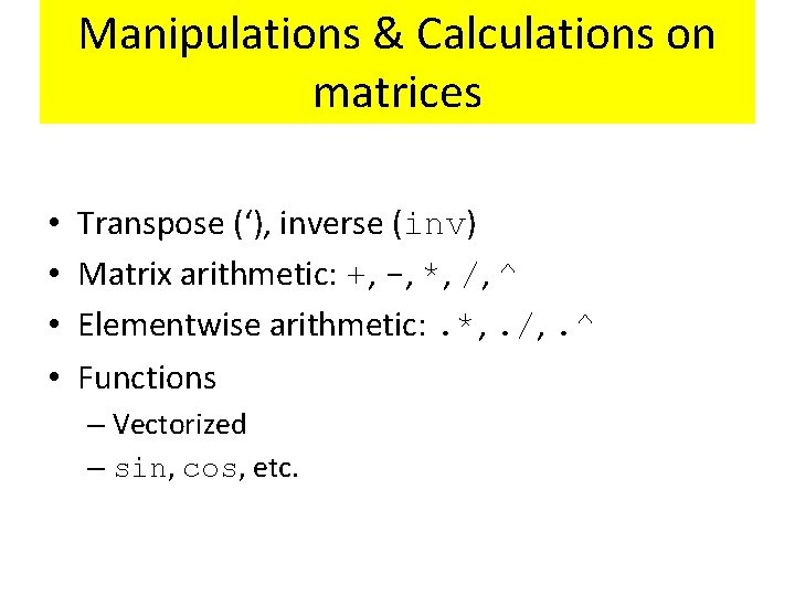
Manipulations & Calculations on matrices • • Transpose (‘), inverse (inv) Matrix arithmetic: +, -, *, /, ^ Elementwise arithmetic: . *, . /, . ^ Functions – Vectorized – sin, cos, etc.
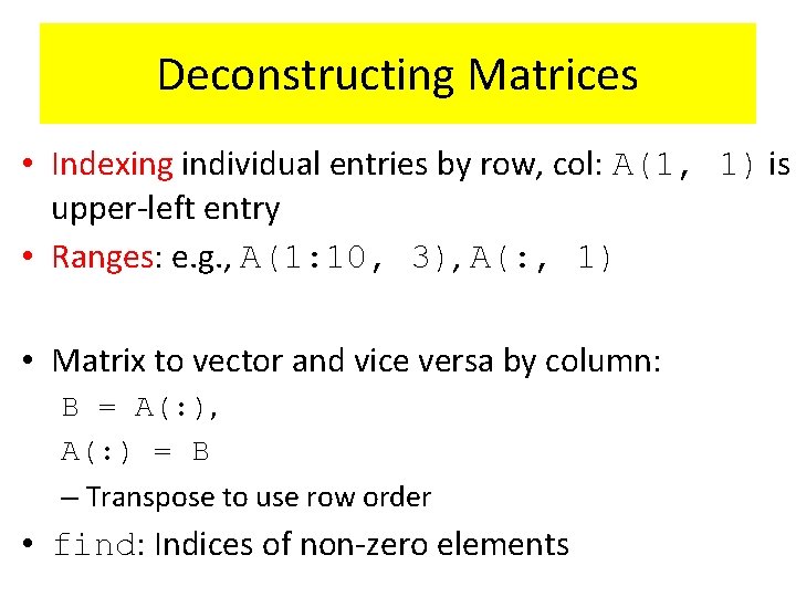
Deconstructing Matrices • Indexing individual entries by row, col: A(1, 1) is upper-left entry • Ranges: e. g. , A(1: 10, 3), A(: , 1) • Matrix to vector and vice versa by column: B = A(: ), A(: ) = B – Transpose to use row order • find: Indices of non-zero elements

Control Structures
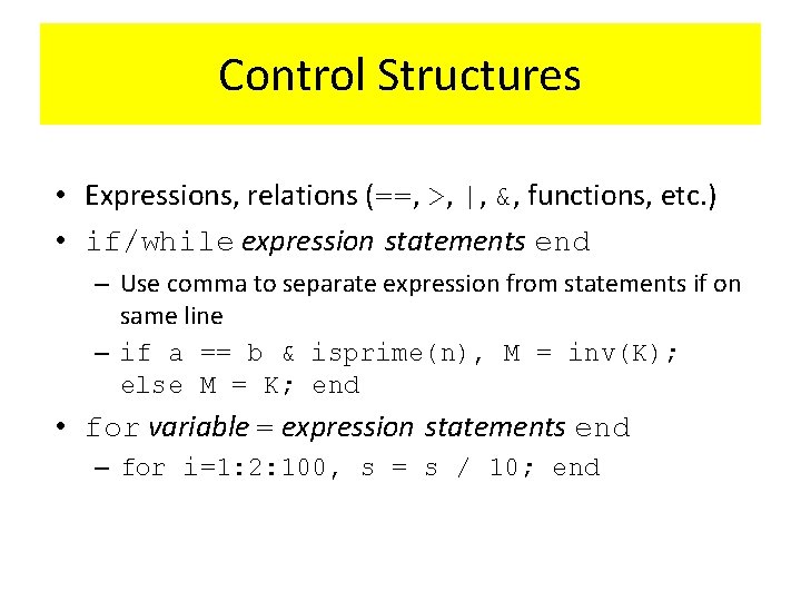
Control Structures • Expressions, relations (==, >, |, &, functions, etc. ) • if/while expression statements end – Use comma to separate expression from statements if on same line – if a == b & isprime(n), M = inv(K); else M = K; end • for variable = expression statements end – for i=1: 2: 100, s = s / 10; end
![function [c, d, e]= pyt(a, b) % returns the hypotenuse in a right angle function [c, d, e]= pyt(a, b) % returns the hypotenuse in a right angle](http://slidetodoc.com/presentation_image_h/229b9dfed465816a40d1835bd514126f/image-19.jpg)
function [c, d, e]= pyt(a, b) % returns the hypotenuse in a right angle % triangle according to Pythagoras theorem. % c is the hypotenuse, % d and e are the two sharp angles c=sqrt(a. ^2+b. ^2); d=atan(b. /a); e=pi/2 -d;
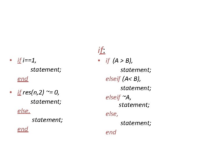
if: • if i==1, statement; end • if res(n, 2) ~= 0, statement; else, statement; end • if (A > B), statement; elseif (A< B), statement; elseif ~A, statement; else, statement; end
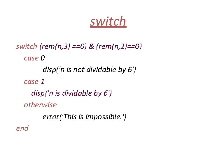
switch (rem(n, 3) ==0) & (rem(n, 2)==0) case 0 disp('n is not dividable by 6') case 1 disp('n is dividable by 6') otherwise error('This is impossible. ') end
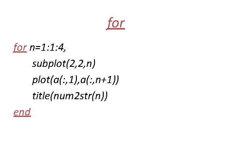
for n=1: 1: 4, subplot(2, 2, n) plot(a(: , 1), a(: , n+1)) title(num 2 str(n)) end
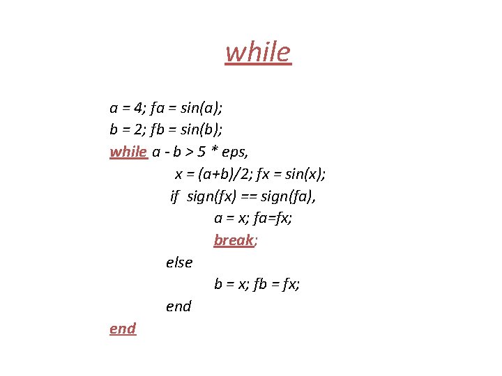
while a = 4; fa = sin(a); b = 2; fb = sin(b); while a - b > 5 * eps, x = (a+b)/2; fx = sin(x); if sign(fx) == sign(fa), a = x; fa=fx; break; else b = x; fb = fx; end
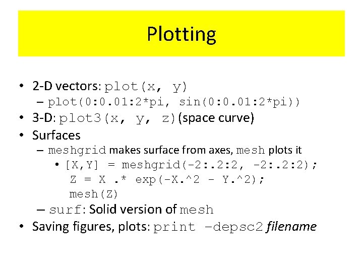
Plotting • 2 -D vectors: plot(x, y) – plot(0: 0. 01: 2*pi, sin(0: 0. 01: 2*pi)) • 3 -D: plot 3(x, y, z)(space curve) • Surfaces – meshgrid makes surface from axes, mesh plots it • [X, Y] = meshgrid(-2: . 2: 2, -2: . 2: 2); Z = X. * exp(-X. ^2 - Y. ^2); mesh(Z) – surf: Solid version of mesh • Saving figures, plots: print –depsc 2 filename
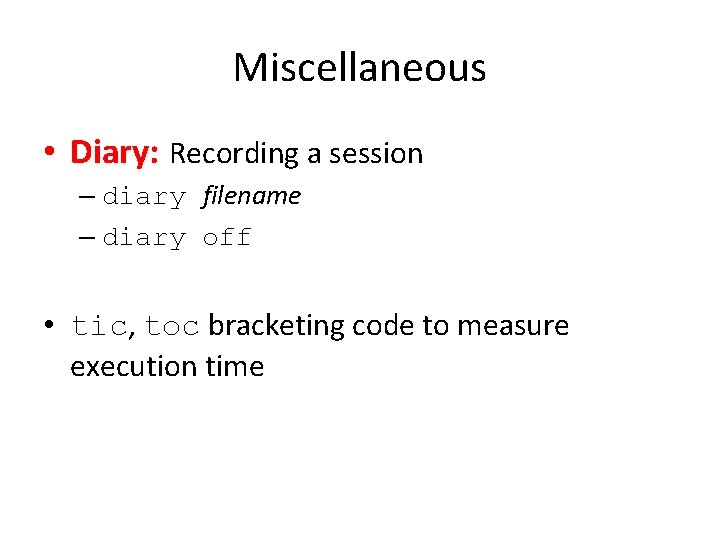
Miscellaneous • Diary: Recording a session – diary filename – diary off • tic, toc bracketing code to measure execution time
Once again: AVOID LOOPS
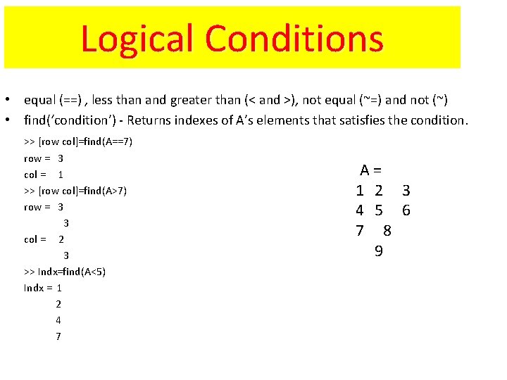
Logical Conditions • equal (==) , less than and greater than (< and >), not equal (~=) and not (~) • find(‘condition’) - Returns indexes of A’s elements that satisfies the condition. >> [row col]=find(A==7) row = 3 col = 1 >> [row col]=find(A>7) row = 3 3 col = 2 3 >> Indx=find(A<5) Indx = 1 2 4 7 A = 1 2 3 4 5 6 7 8 9

Flow Control • Flow control in MATLAB - if, else and elseif statements (row=1, 2, 3 col=1, 2, 3) if row==col A(row, col)=1; elseif abs(row-col)==1 A(row, col)=2; else A(row, col)=0; end A = 1 2 0 2 1
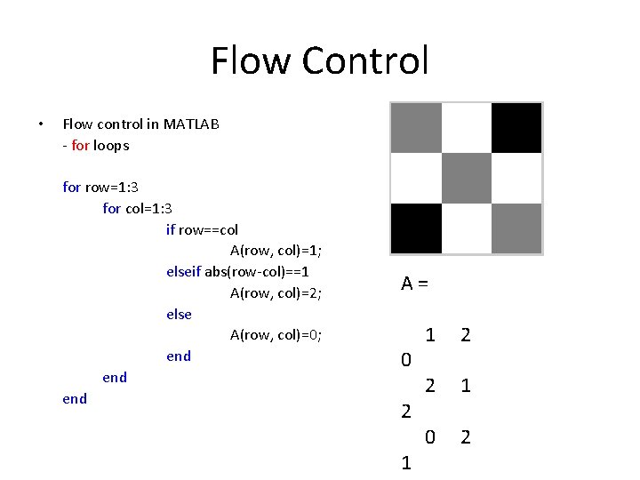
Flow Control • Flow control in MATLAB - for loops for row=1: 3 for col=1: 3 if row==col A(row, col)=1; elseif abs(row-col)==1 A(row, col)=2; else A(row, col)=0; end end A = 1 2 0 2 1
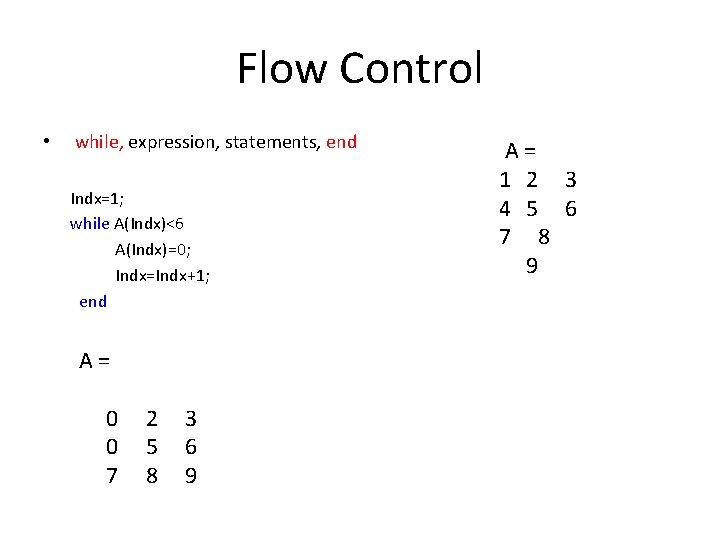
Flow Control • while, expression, statements, end Indx=1; while A(Indx)<6 A(Indx)=0; Indx=Indx+1; end A = 0 2 3 0 5 6 7 8 9 A = 1 2 3 4 5 6 7 8 9
M-Files • Any text file ending in “. m” • Use path or addpath to tell Matlab where code is (non-persistent? ) • Script: Collection of command line statements • Function: Take argument(s), return value(s). First line defines: – function y = foo(A) – function [x, y] = foo 2(a, M, N) • Comment: Start line with %
Working with M-Files • M-files can be scripts that simply execute a series of MATLAB statements, or they can be functions that also accept input arguments and produce output. • MATLAB functions: – Are useful for extending the MATLAB language for your application. – Can accept input arguments and return output arguments. – Store variables in a workspace internal to the function.
![Working with M-Files Create a new empty m-file function B=test(I) [row col]=size(I) for r=1: Working with M-Files Create a new empty m-file function B=test(I) [row col]=size(I) for r=1:](http://slidetodoc.com/presentation_image_h/229b9dfed465816a40d1835bd514126f/image-33.jpg)
Working with M-Files Create a new empty m-file function B=test(I) [row col]=size(I) for r=1: row for c=1: col if r==c A(r, c)=1; elseif abs(r-c)==1 A(r, c)=2; else A(r, c)=0; end end B=A; •
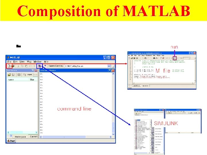
Composition of MATLAB 34

Examples Try these MATRIX AND VECTOR OPERATIONS This is how we can define a vector >> v=[1, 2, 3] Matlab prints out the following v = 1 2 3 Similarly we can define a matrix >> M= [ 1 2 3; 4 5 6; 7 8 9] The result is: M = 1 2 3 4 5 6 7 8 9 If you want to suppress the Mat. Lab output then you need to finish the line with semicolon as follows. >>M= [ 1 2 3; 4 5 6; 7 8 9];
Projection Say you want to extract some rows and columns of a matrix. This is called a projection. We simply give the subset of rows and columns as parameters, as follows >> M 11=M(2: 3 , 2: 3) M 11 = 5 6 8 9 To specify all elements in a given dimension one can use ': ‘ So to get all rows but just columns 1 and 2, we type >> A= M( : , 1: 2) A = 1 2 4 5 7 8
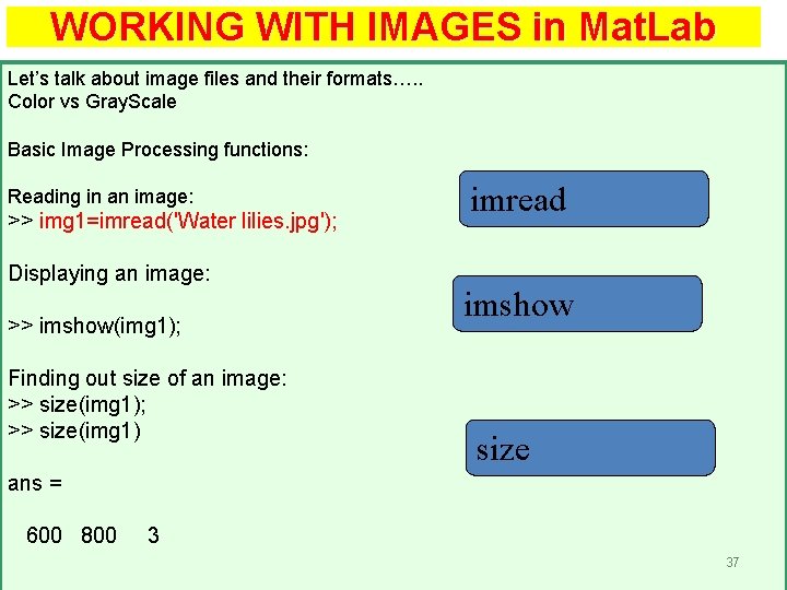
WORKING WITH IMAGES in Mat. Lab Let’s talk about image files and their formats…. . Color vs Gray. Scale Basic Image Processing functions: Reading in an image: >> img 1=imread('Water lilies. jpg'); Displaying an image: >> imshow(img 1); Finding out size of an image: >> size(img 1); >> size(img 1) imread imshow size ans = 600 800 3 37
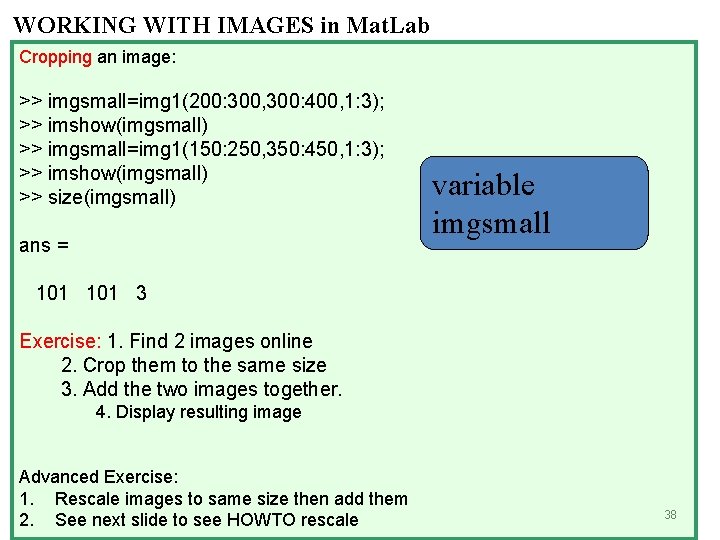
WORKING WITH IMAGES in Mat. Lab Cropping an image: >> imgsmall=img 1(200: 300, 300: 400, 1: 3); >> imshow(imgsmall) >> imgsmall=img 1(150: 250, 350: 450, 1: 3); >> imshow(imgsmall) >> size(imgsmall) ans = variable imgsmall 101 3 Exercise: 1. Find 2 images online 2. Crop them to the same size 3. Add the two images together. 4. Display resulting image Advanced Exercise: 1. Rescale images to same size then add them 2. See next slide to see HOWTO rescale 38
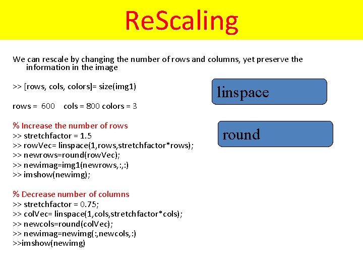
Re. Scaling We can rescale by changing the number of rows and columns, yet preserve the information in the image >> [rows, colors]= size(img 1) rows = 600 cols = 800 colors = 3 % Increase the number of rows >> stretchfactor = 1. 5 >> row. Vec= linspace(1, rows, stretchfactor*rows); >> newrows=round(row. Vec); >> newimag=img 1(newrows, : ) >> imshow(newimg); % Decrease number of columns >> stretchfactor = 0. 75; >> col. Vec= linspace(1, cols, stretchfactor*cols); >> newcols=round(col. Vec); >> newimag=newimg(: , newcols, : ) >>imshow(newimg) linspace round
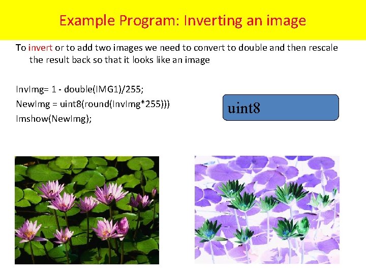
Example Program: Inverting an image To invert or to add two images we need to convert to double and then rescale invert the result back so that it looks like an image Inv. Img= 1 - double(IMG 1)/255; New. Img = uint 8(round(Inv. Img*255))) Imshow(New. Img); uint 8 40
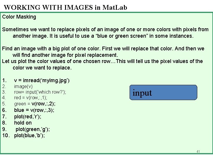
WORKING WITH IMAGES in Mat. Lab Color Masking Sometimes we want to replace pixels of an image of one or more colors with pixels from another image. It is useful to use a “blue or green screen” in some instances. Find an image with a big plot of one color. First we will replace that color. And then we will find another image for pixel replacement. Let us plot the color values of one chosen row…This will tell us the pixel values of the color we want to replace. 1. v = imread(‘myimg. jpg’) 2. 3. 4. 5. image(v) row= input(‘which row? ’); red = v(row, : , 1); green = v(row, : , 2); 6. 7. 8. 9. 10. blue = v(row, : , 3); plot(red, ’r’); hold on plot(green, ’g’); plot(blue, ’b’); input 41
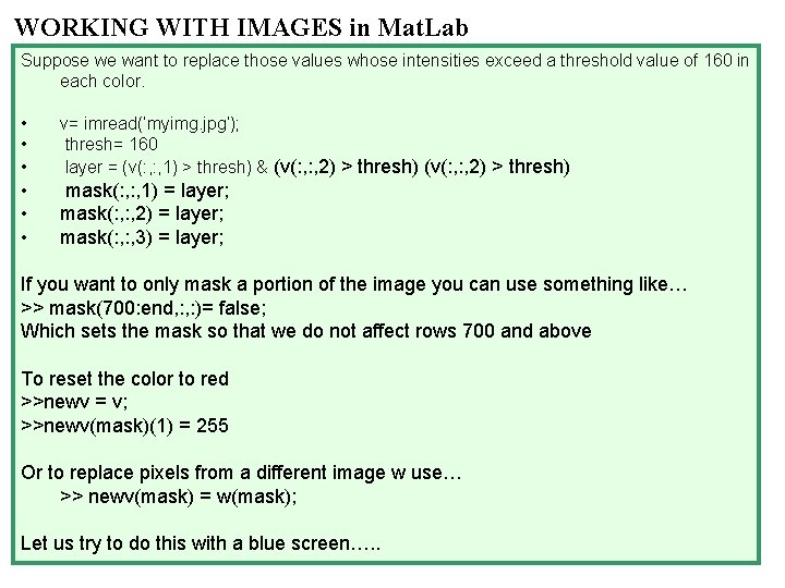
WORKING WITH IMAGES in Mat. Lab Suppose we want to replace those values whose intensities exceed a threshold value of 160 in each color. • • • v= imread(‘myimg. jpg’); thresh= 160 layer = (v(: , 1) > thresh) & (v(: , : , 2) > thresh) • • • mask(: , 1) = layer; mask(: , 2) = layer; mask(: , 3) = layer; If you want to only mask a portion of the image you can use something like… >> mask(700: end, : )= false; Which sets the mask so that we do not affect rows 700 and above To reset the color to red >>newv = v; >>newv(mask)(1) = 255 Or to replace pixels from a different image w use… >> newv(mask) = w(mask); Let us try to do this with a blue screen…. .
Histograms
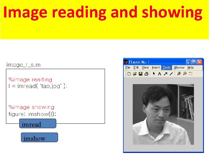
Image reading and showing imread imshow
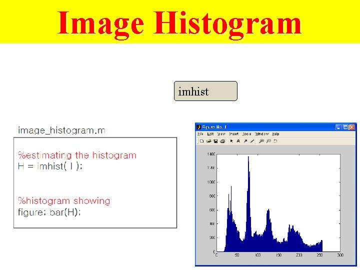
Image Histogram imhist 45
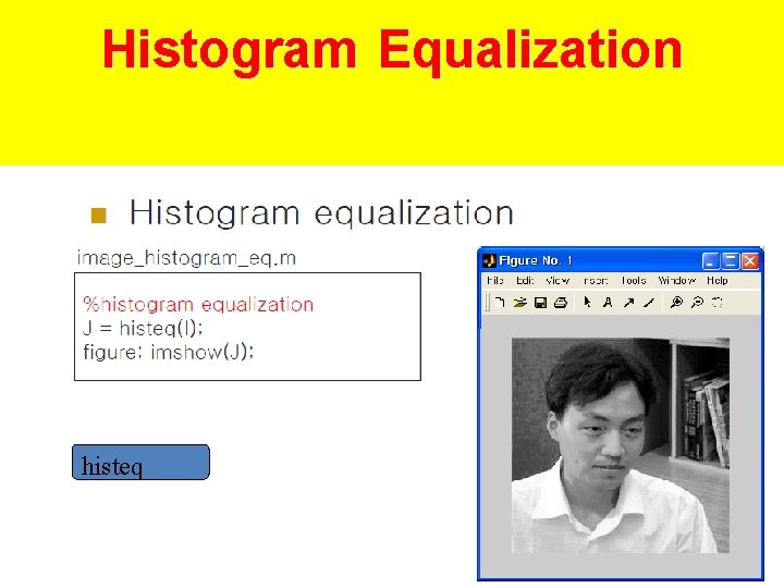
Histogram Equalization histeq
Noise
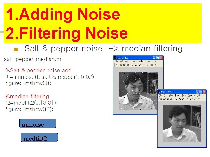
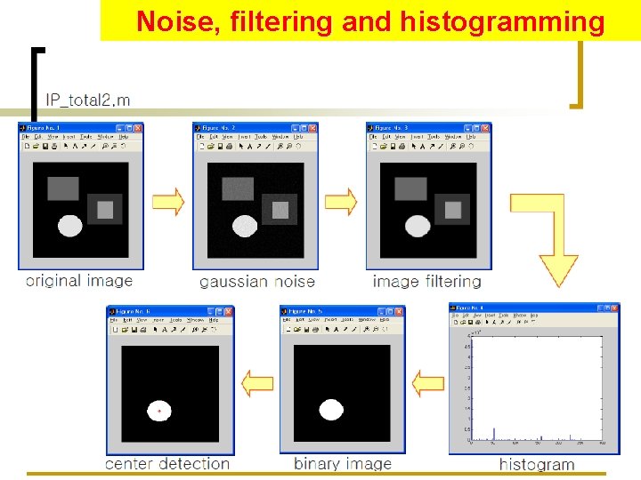
1. Adding Noise 2. Filtering Noise imnoise medfilt 2
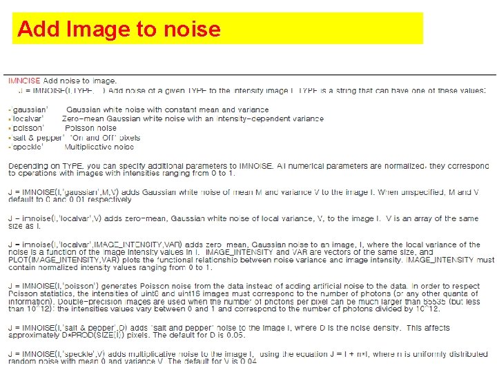
Add Image to noise 50
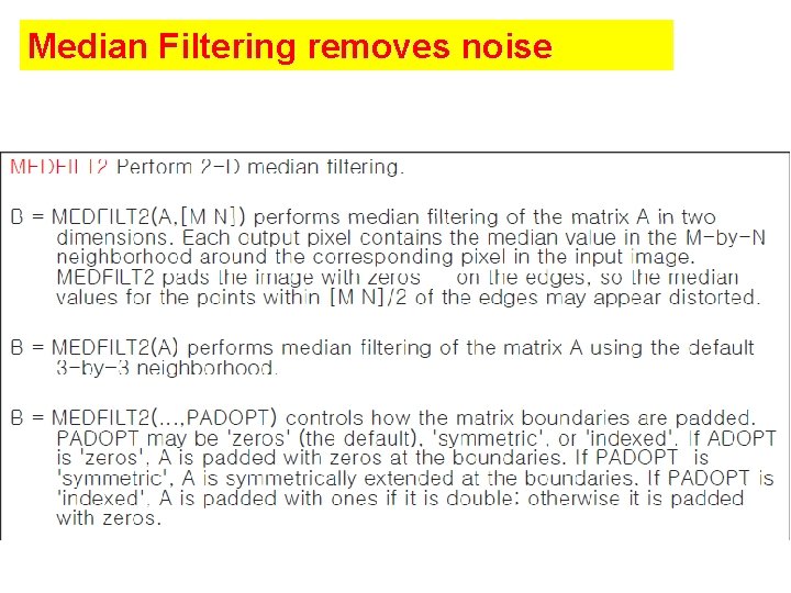
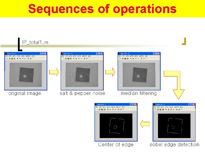
Median Filtering removes noise
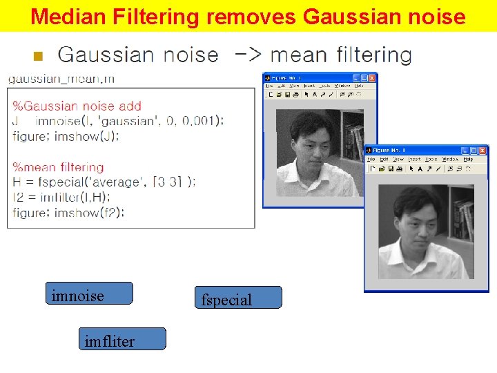
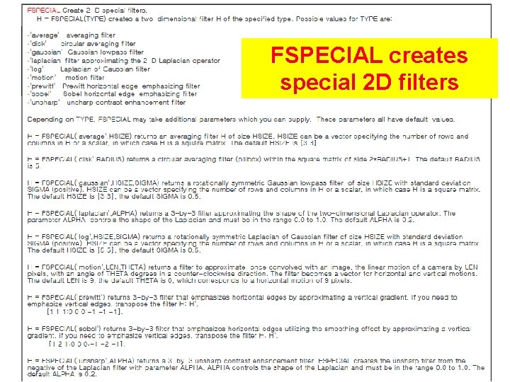
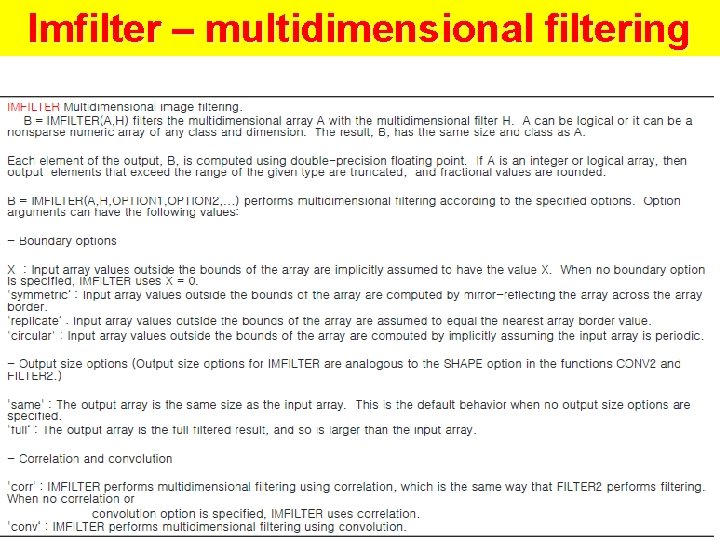
Median Filtering removes Gaussian noise imfliter fspecial
FSPECIAL creates special 2 D filters 53
Imfilter – multidimensional filtering 54
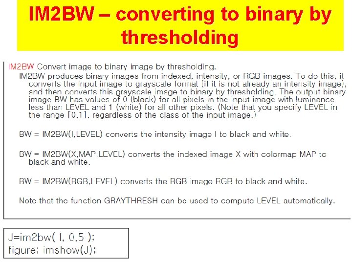
Thresholding
Thresholding
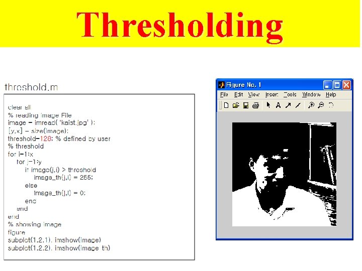
IM 2 BW – converting to binary by thresholding 57
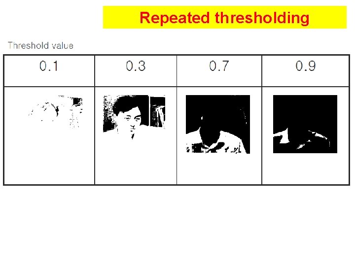
Repeated thresholding
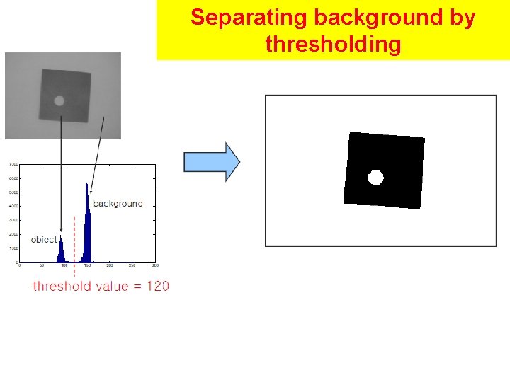
Separating background by thresholding
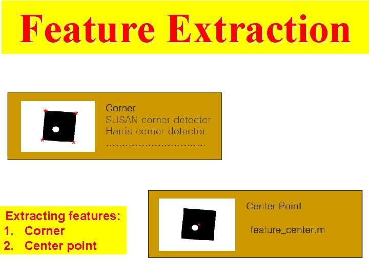
Feature Extraction Extracting features: 1. Corner 2. Center point
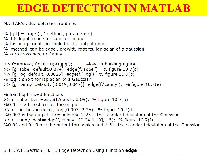
Edge Detection
Edge Detection edge Example of kernel-based filtering - Sobel
Edge, Sobel and Prewitt 63
Roberts, Laplacian, Zero-cross, Canny edge detection methods 64
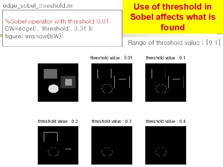
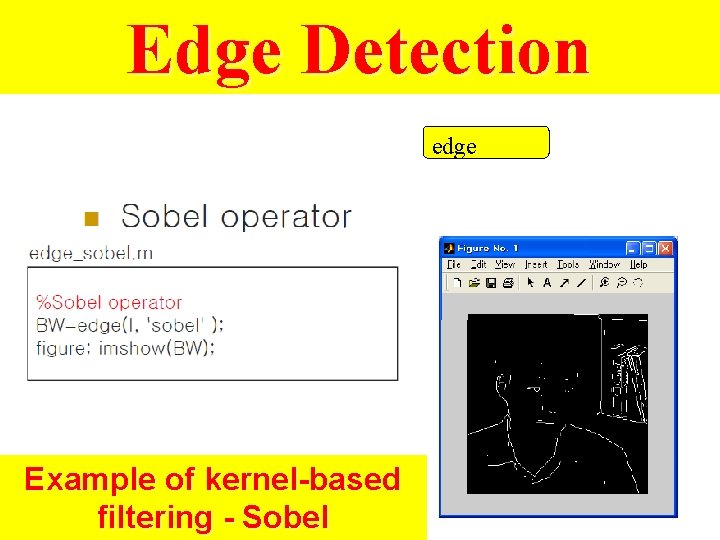
Use of threshold in Sobel affects what is found 65
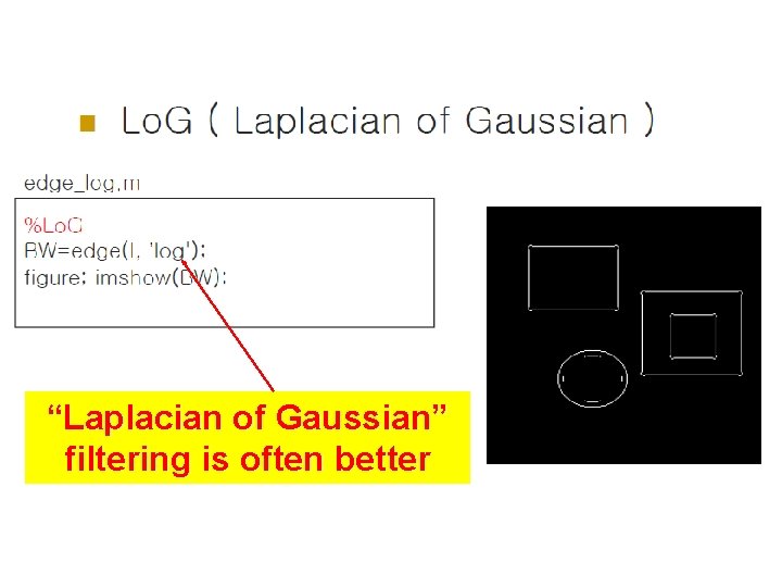
“Laplacian of Gaussian” filtering is often better
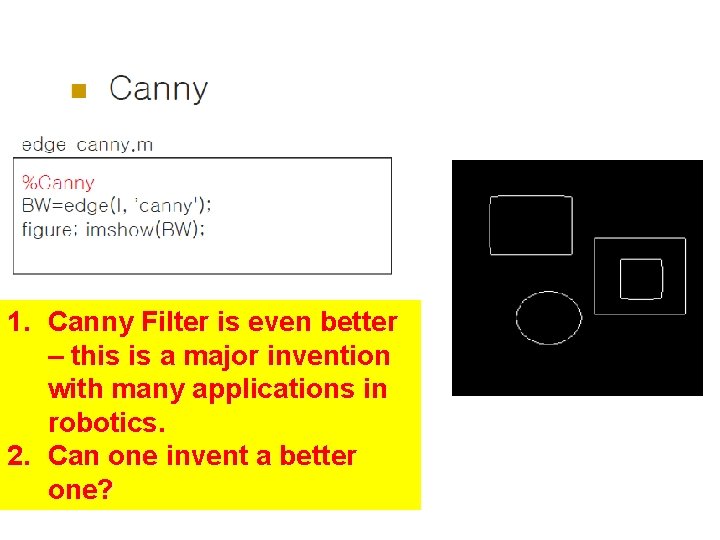
1. Canny Filter is even better – this is a major invention with many applications in robotics. 2. Can one invent a better one?
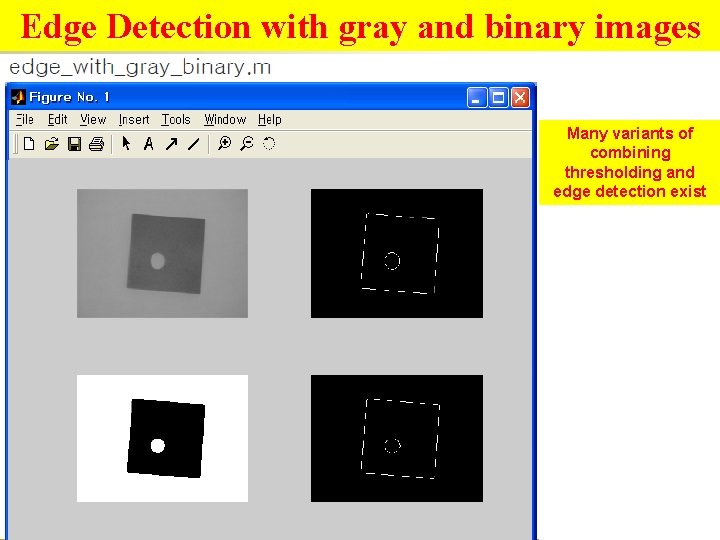
Edge Detection with gray and binary images Many variants of combining thresholding and edge detection exist
EDGE DETECTION IN MATLAB

Hough Transform
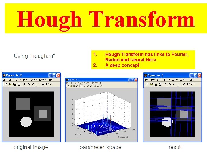
Hough Transform 1. 2. Hough Transform has links to Fourier, Radon and Neural Nets. A deep concept
Camera Calibration
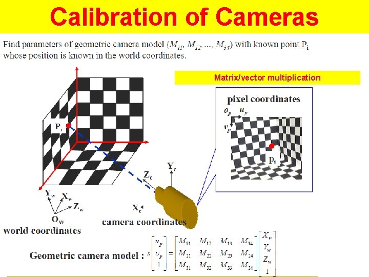
Calibration of Cameras Matrix/vector multiplication
Sequences of operations 74
Noise, filtering and histogramming 75
Fourier Transform in MATLAB
Other data MATLAB can also handle • Movies • 3 D objects • …
Sources 1. 2. 3. 4. 5. 6. Rolf Lakaemper Fred Annexstein Jason Rife Hyunki Lee Amin Allalou www. cis. udel. edu/~cer/arv
- Slides: 78