Matlab Training Sessions 6 7 Plotting Course Outline

Matlab Training Sessions 6, 7: Plotting

Course Outline Weeks: 1. Introduction to Matlab and its Interface (Jan 13 2009) 2. Fundamentals (Operators) 3. Fundamentals (Flow) 4. Importing Data 5. Functions and M-Files 6. Plotting (2 D and 3 D) 7. Statistical Tools in Matlab 8. Analysis and Data Structures Course Website: http: //www. queensu. ca/neurosci/matlab. php

Week 5 Lecture Outline Plotting Data A. Basics B. Generating data C. 2 D Plots (Line, Scatter, Bar) D. Plot Features

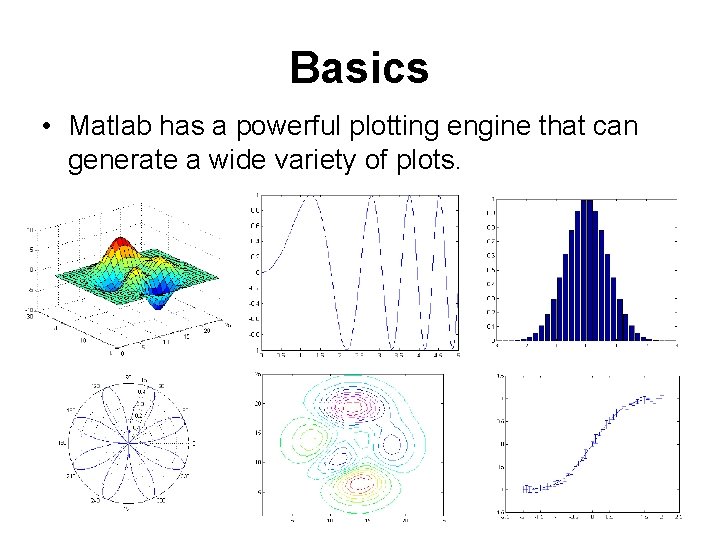
Basics • Matlab has a powerful plotting engine that can generate a wide variety of plots.

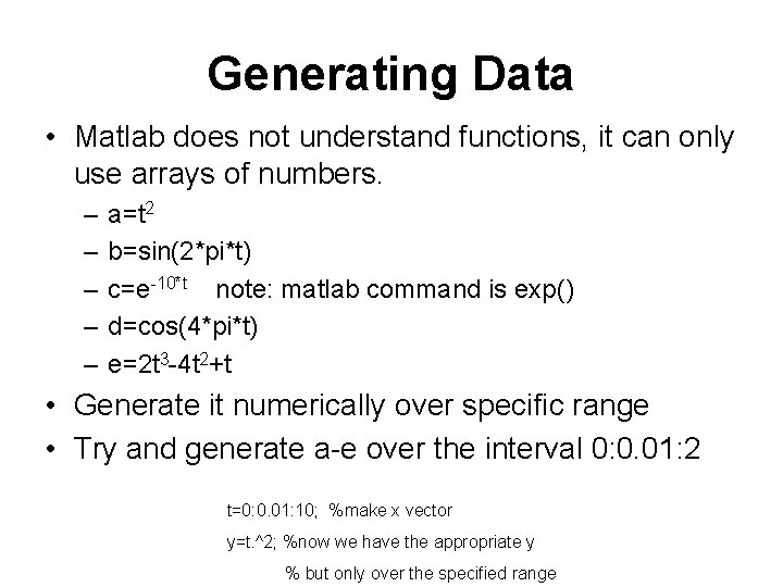
Generating Data • Matlab does not understand functions, it can only use arrays of numbers. – – – a=t 2 b=sin(2*pi*t) c=e-10*t note: matlab command is exp() d=cos(4*pi*t) e=2 t 3 -4 t 2+t • Generate it numerically over specific range • Try and generate a-e over the interval 0: 0. 01: 2 t=0: 0. 01: 10; %make x vector y=t. ^2; %now we have the appropriate y % but only over the specified range

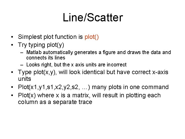
Line/Scatter • Simplest plot function is plot() • Try typing plot(y) – Matlab automatically generates a figure and draws the data and connects its lines – Looks right, but the x axis units are incorrect • Type plot(x, y), will look identical but have correct x-axis units • Plot(x 1, y 1, s 1, x 2, y 2, s 2, …) many plots in one command • Plot(x) where x is a matrix, will result in plotting each column as a separate trace

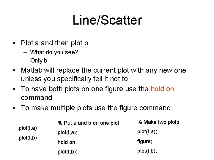
Line/Scatter • Plot a and then plot b – What do you see? – Only b • Matlab will replace the current plot with any new one unless you specifically tell it not to • To have both plots on one figure use the hold on command • To make multiple plots use the figure command plot(t, a) plot(t, b) % Put a and b on one plot % Make two plots plot(t, a); hold on; figure; plot(t, b);

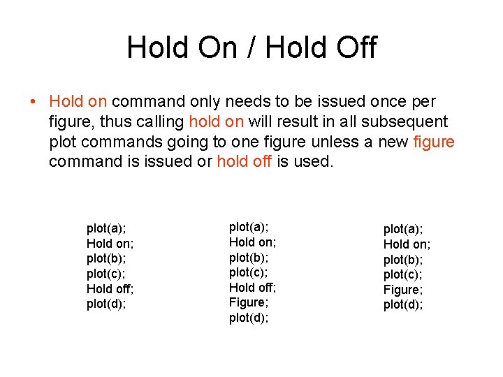
Hold On / Hold Off • Hold on command only needs to be issued once per figure, thus calling hold on will result in all subsequent plot commands going to one figure unless a new figure command is issued or hold off is used. plot(a); Hold on; plot(b); plot(c); Hold off; plot(d); plot(a); Hold on; plot(b); plot(c); Hold off; Figure; plot(d); plot(a); Hold on; plot(b); plot(c); Figure; plot(d);

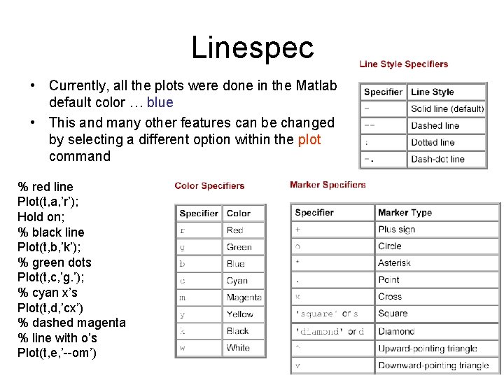
Linespec • Currently, all the plots were done in the Matlab default color … blue • This and many other features can be changed by selecting a different option within the plot command % red line Plot(t, a, ’r’); Hold on; % black line Plot(t, b, ’k’); % green dots Plot(t, c, ’g. ’); % cyan x’s Plot(t, d, ’cx’) % dashed magenta % line with o’s Plot(t, e, ’--om’)

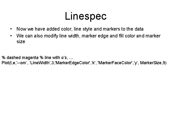
Linespec • Now we have added color, line style and markers to the data • We can also modify line width, marker edge and fill color and marker size % dashed magenta % line with o’s, … Plot(t, e, ’--om’, ‘Line. Width’, 3, 'Marker. Edge. Color', ‘k‘, 'Marker. Face. Color', ‘y‘, Marker. Size, 9)

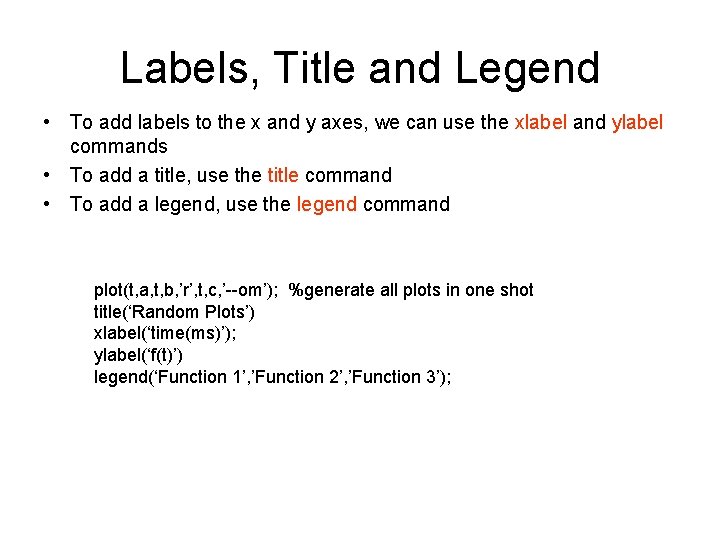
Labels, Title and Legend • To add labels to the x and y axes, we can use the xlabel and ylabel commands • To add a title, use the title command • To add a legend, use the legend command plot(t, a, t, b, ’r’, t, c, ’--om’); %generate all plots in one shot title(‘Random Plots’) xlabel(‘time(ms)’); ylabel(‘f(t)’) legend(‘Function 1’, ’Function 2’, ’Function 3’);

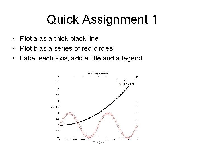
Quick Assignment 1 • Plot a as a thick black line • Plot b as a series of red circles. • Label each axis, add a title and a legend

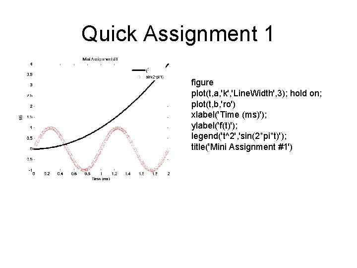
Quick Assignment 1 figure plot(t, a, 'k', 'Line. Width', 3); hold on; plot(t, b, 'ro') xlabel('Time (ms)'); ylabel('f(t)'); legend('t^2', 'sin(2*pi*t)'); title('Mini Assignment #1')

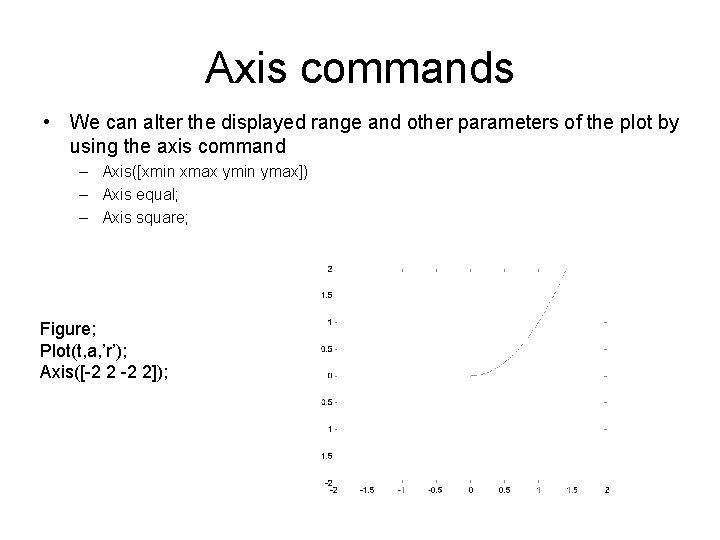
Axis commands • We can alter the displayed range and other parameters of the plot by using the axis command – Axis([xmin xmax ymin ymax]) – Axis equal; – Axis square; Figure; Plot(t, a, ’r’); Axis([-2 2]);

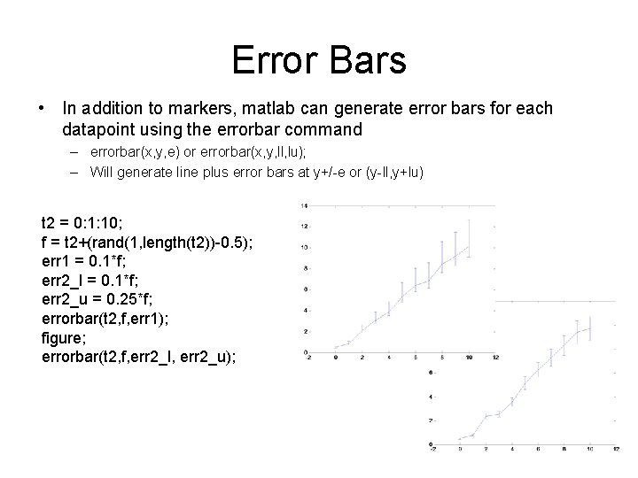
Error Bars • In addition to markers, matlab can generate error bars for each datapoint using the errorbar command – errorbar(x, y, e) or errorbar(x, y, ll, lu); – Will generate line plus error bars at y+/-e or (y-ll, y+lu) t 2 = 0: 1: 10; f = t 2+(rand(1, length(t 2))-0. 5); err 1 = 0. 1*f; err 2_l = 0. 1*f; err 2_u = 0. 25*f; errorbar(t 2, f, err 1); figure; errorbar(t 2, f, err 2_l, err 2_u);

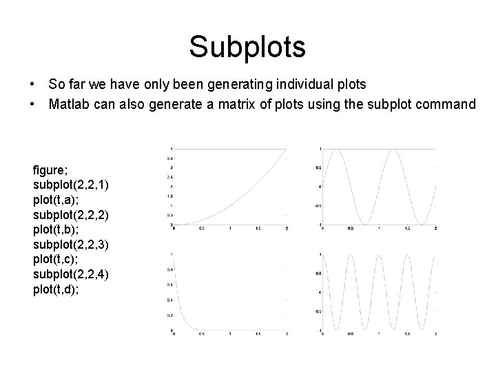
Subplots • So far we have only been generating individual plots • Matlab can also generate a matrix of plots using the subplot command figure; subplot(2, 2, 1) plot(t, a); subplot(2, 2, 2) plot(t, b); subplot(2, 2, 3) plot(t, c); subplot(2, 2, 4) plot(t, d);

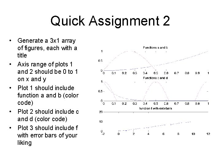
Quick Assignment 2 • Generate a 3 x 1 array of figures, each with a title • Axis range of plots 1 and 2 should be 0 to 1 on x and y • Plot 1 should include function a and b (color code) • Plot 2 should include c and d (color code) • Plot 3 should include f with error bars of your liking

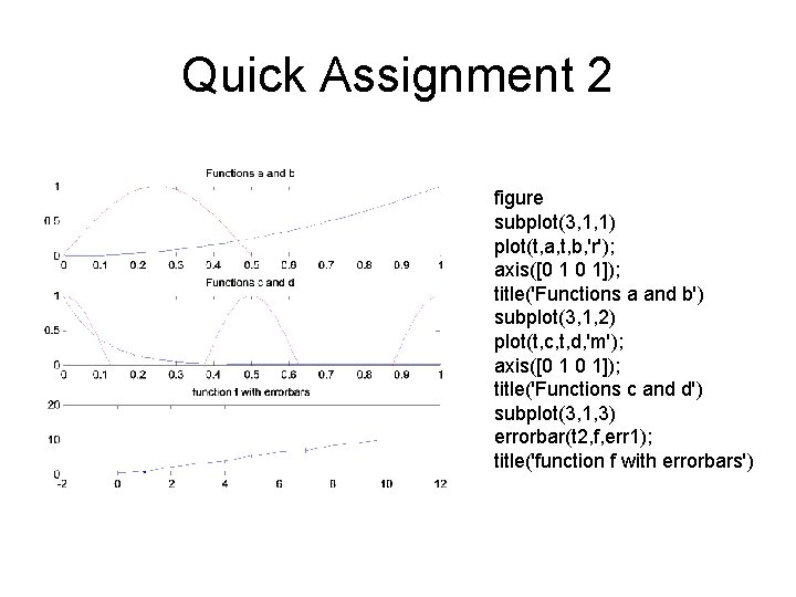
Quick Assignment 2 figure subplot(3, 1, 1) plot(t, a, t, b, 'r'); axis([0 1 0 1]); title('Functions a and b') subplot(3, 1, 2) plot(t, c, t, d, 'm'); axis([0 1 0 1]); title('Functions c and d') subplot(3, 1, 3) errorbar(t 2, f, err 1); title('function f with errorbars')

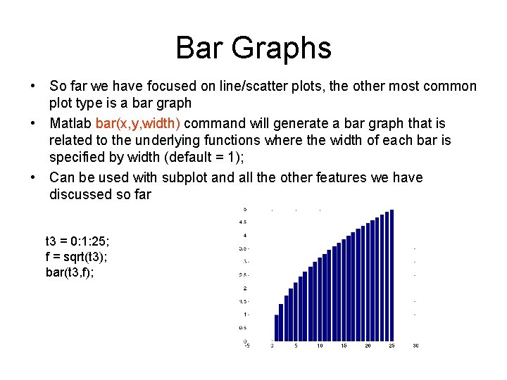
Bar Graphs • So far we have focused on line/scatter plots, the other most common plot type is a bar graph • Matlab bar(x, y, width) command will generate a bar graph that is related to the underlying functions where the width of each bar is specified by width (default = 1); • Can be used with subplot and all the other features we have discussed so far t 3 = 0: 1: 25; f = sqrt(t 3); bar(t 3, f);

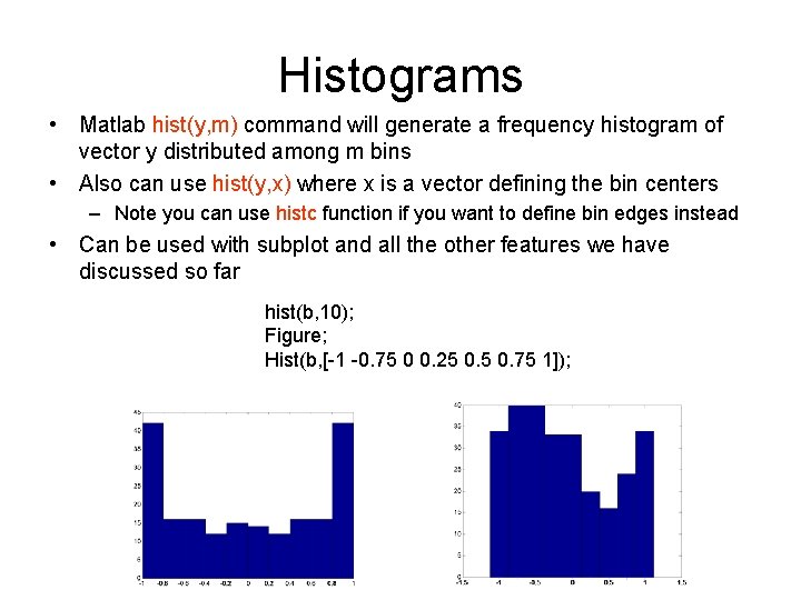
Histograms • Matlab hist(y, m) command will generate a frequency histogram of vector y distributed among m bins • Also can use hist(y, x) where x is a vector defining the bin centers – Note you can use histc function if you want to define bin edges instead • Can be used with subplot and all the other features we have discussed so far hist(b, 10); Figure; Hist(b, [-1 -0. 75 0 0. 25 0. 75 1]);

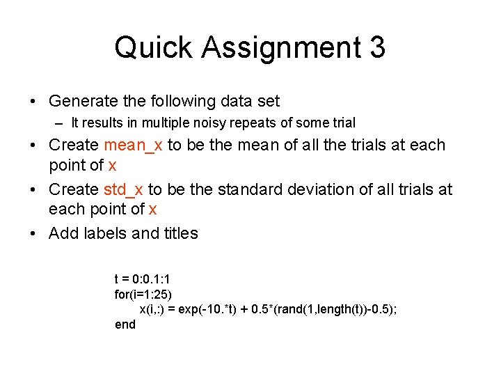
Quick Assignment 3 • Generate the following data set – It results in multiple noisy repeats of some trial • Create mean_x to be the mean of all the trials at each point of x • Create std_x to be the standard deviation of all trials at each point of x • Add labels and titles t = 0: 0. 1: 1 for(i=1: 25) x(i, : ) = exp(-10. *t) + 0. 5*(rand(1, length(t))-0. 5); end

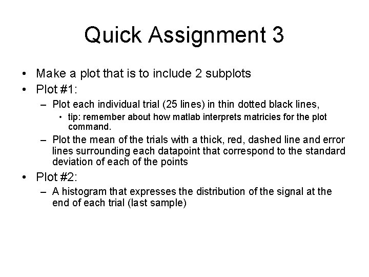
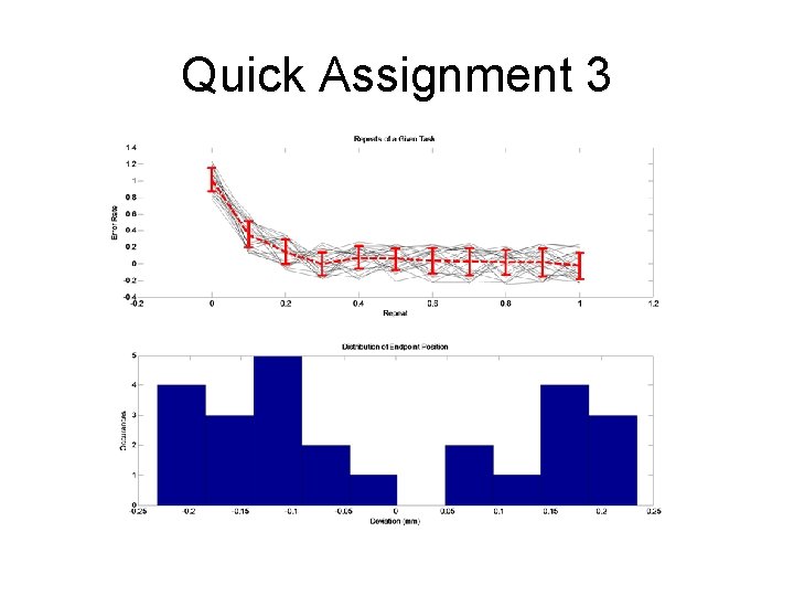
Quick Assignment 3 • Make a plot that is to include 2 subplots • Plot #1: – Plot each individual trial (25 lines) in thin dotted black lines, • tip: remember about how matlab interprets matricies for the plot command. – Plot the mean of the trials with a thick, red, dashed line and error lines surrounding each datapoint that correspond to the standard deviation of each of the points • Plot #2: – A histogram that expresses the distribution of the signal at the end of each trial (last sample)

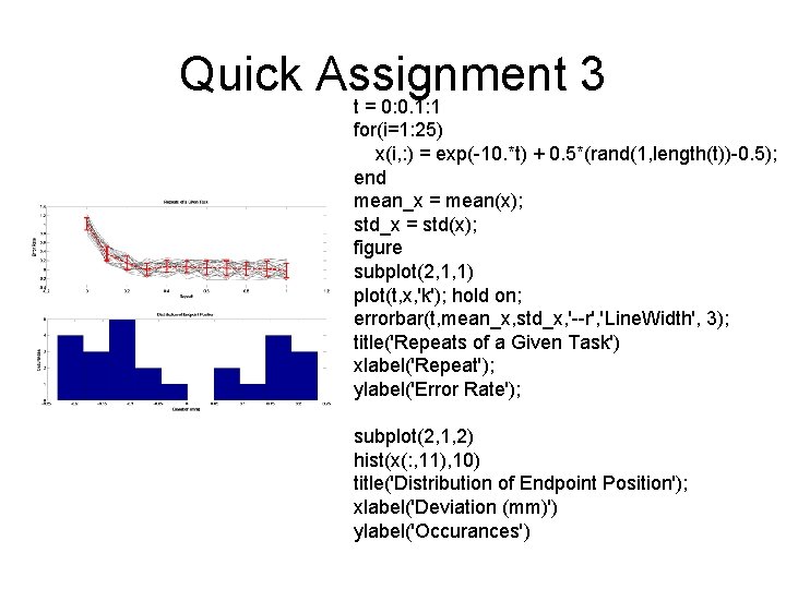
Quick Assignment 3 t = 0: 0. 1: 1 for(i=1: 25) x(i, : ) = exp(-10. *t) + 0. 5*(rand(1, length(t))-0. 5); end mean_x = mean(x); std_x = std(x); figure subplot(2, 1, 1) plot(t, x, 'k'); hold on; errorbar(t, mean_x, std_x, '--r', 'Line. Width', 3); title('Repeats of a Given Task') xlabel('Repeat'); ylabel('Error Rate'); subplot(2, 1, 2) hist(x(: , 11), 10) title('Distribution of Endpoint Position'); xlabel('Deviation (mm)') ylabel('Occurances')

Quick Assignment 3

Recap • Learned about basic 2 D plot functions – plot, bar, hist • Dealing with multiple plots and graphs – Hold, figure, subplot • Discussed adding features to graphs – Xlabel, title, legend, …

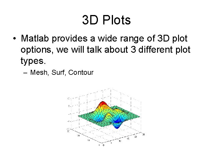
3 D Plots • Matlab provides a wide range of 3 D plot options, we will talk about 3 different plot types. – Mesh, Surf, Contour

Dataset • Try [x, y, z] = peaks(25) – Does this work? • If not, lets create an arbitrary dataset – x=-10: 10; y = -10: 10; z=x. ^2’*y. ^2;

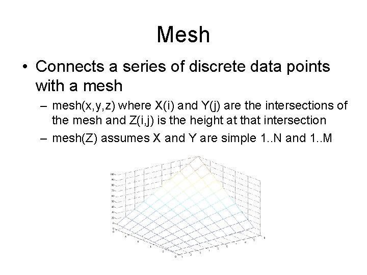
Mesh • Connects a series of discrete data points with a mesh – mesh(x, y, z) where X(i) and Y(j) are the intersections of the mesh and Z(i, j) is the height at that intersection – mesh(Z) assumes X and Y are simple 1. . N and 1. . M

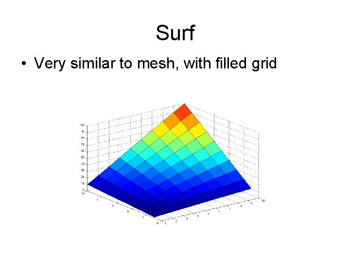
Surf • Very similar to mesh, with filled grid

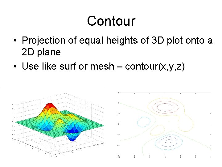
Contour • Projection of equal heights of 3 D plot onto a 2 D plane • Use like surf or mesh – contour(x, y, z)

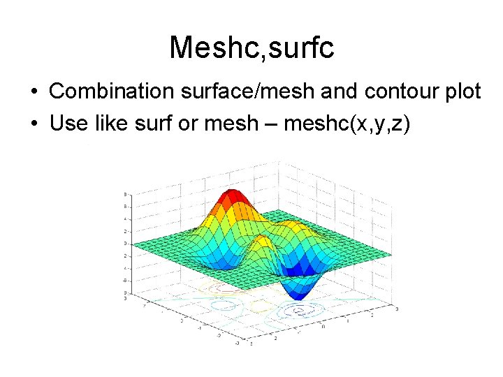
Meshc, surfc • Combination surface/mesh and contour plot • Use like surf or mesh – meshc(x, y, z)

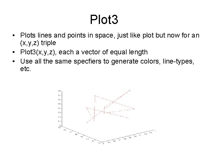
Plot 3 • Plots lines and points in space, just like plot but now for an (x, y, z) triple • Plot 3(x, y, z), each a vector of equal length • Use all the same specfiers to generate colors, line-types, etc.

Plot commands • Note that almost all 2 D plotting commands such as xlabel, ylabel, title will still work in 3 D plots • 3 D plots can be added as subplots just like any other plot type • Some other special features and functions exist…

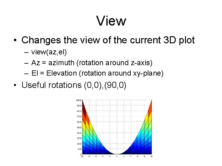
View • Changes the view of the current 3 D plot – view(az, el) – Az = azimuth (rotation around z-axis) – El = Elevation (rotation around xy-plane) • Useful rotations (0, 0), (90, 0)

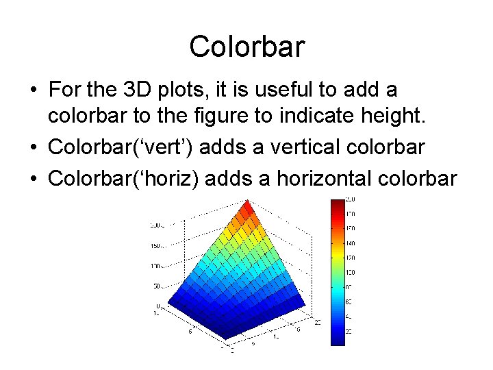
Colorbar • For the 3 D plots, it is useful to add a colorbar to the figure to indicate height. • Colorbar(‘vert’) adds a vertical colorbar • Colorbar(‘horiz) adds a horizontal colorbar

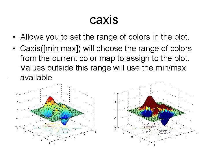
caxis • Allows you to set the range of colors in the plot. • Caxis([min max]) will choose the range of colors from the current color map to assign to the plot. Values outside this range will use the min/max available

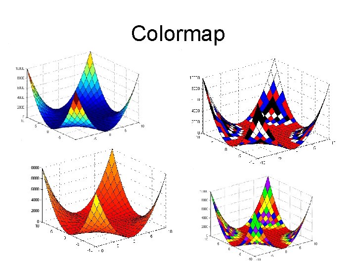
Colormap • Plenty of other controls to personalize the plot – colormap_name sets to new map – Colormap (sets the types of colors that appear in 3 D plot). These can be custom of one of several premade – bone Hsv, jet, autumn, vga, summer, … – See help graph 3 D for more – Use colormapeditor function for graphical selection of color map

Colormap

Next Week • Basic Stats / Basic Matlab wrap up

Getting Help and Documentation Digital 1. Accessible Help from the Matlab Start Menu 2. Updated online help from the Matlab Mathworks website: http: //www. mathworks. com/access/helpdesk/help/techdoc/matlab. html 3. Matlab command prompt function lookup 4. Built in Demo’s 5. Websites Hard Copy 3. Books, Guides, Reference The Student Edition of Matlab pub. Mathworks Inc.