MATLAB Ordinary Differential Equations Part I Greg Reese

MATLAB Ordinary Differential Equations – Part I Greg Reese, Ph. D Research Computing Support Group Academic Technology Services Miami University September 2013

MATLAB Ordinary Differential Equations – Part I © 2010 -2013 Greg Reese. All rights reserved 2

ODE Ordinary Differential Equation (ODE) Differential Equation – an equation with an unknown function and some of its derivatives Ordinary – the function depends on one variable only 3

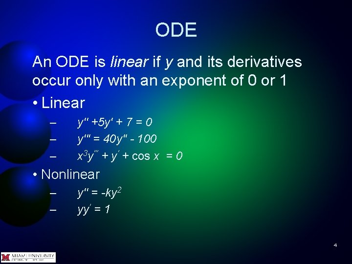
ODE An ODE is linear if y and its derivatives occur only with an exponent of 0 or 1 • Linear – – – y'' +5 y' + 7 = 0 y''' = 40 y'' - 100 x 3 y''' + y' + cos x = 0 • Nonlinear – – y'' = -ky 2 yy' = 1 4

ODE Ordinary Differential Equation (ODE) • Independent variable often denoted as t and referred to as "time" • Unknown function often denoted as y(t) • The derivative of y with respect to t is denoted as y', the second derivative as y'', and so on 5

ODE The degree of the highest derivative in a differential equation is that equation's order, e. g. , • y' = ky first order • y'' + 2 y' + 3 y = sin(t) second order • y''' +2 y'' + 2 y + 2 =40 third order All of MATLAB's ODE solvers take only first order systems of equations. Not a severe restriction though 6

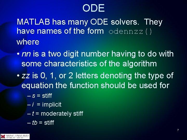
ODE MATLAB has many ODE solvers. They have names of the form odennzz() where • nn is a two digit number having to do with some characteristics of the algorithm • zz is 0, 1, or 2 letters denoting the type of equation the function should be used for – s = stiff – i = implicit – t = moderately stiff – tb = stiff 7

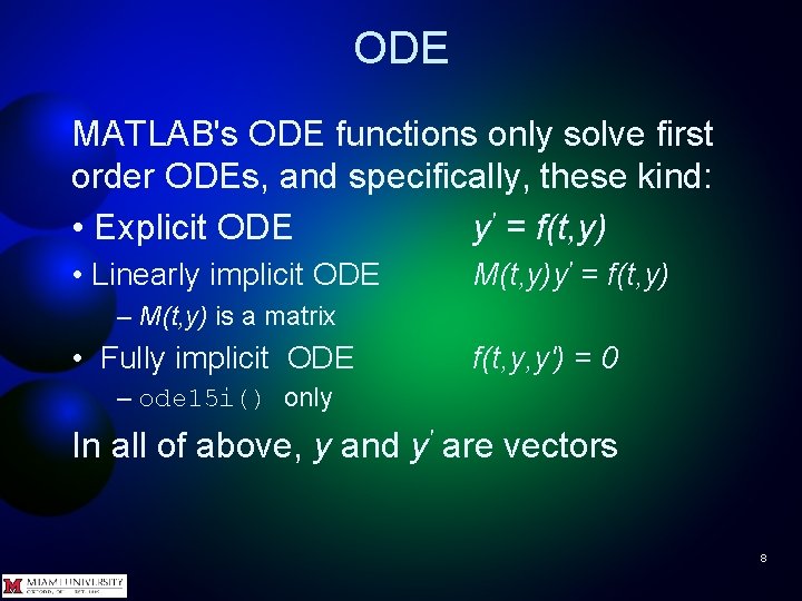
ODE MATLAB's ODE functions only solve first order ODEs, and specifically, these kind: • Explicit ODE y' = f(t, y) • Linearly implicit ODE M(t, y)y' = f(t, y) – M(t, y) is a matrix • Fully implicit ODE f(t, y, y') = 0 – ode 15 i() only In all of above, y and y' are vectors 8

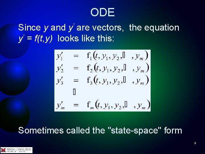
ODE Since y and y' are vectors, the equation y' = f(t, y) looks like this: Sometimes called the "state-space" form 9

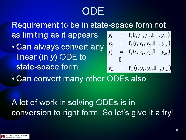
ODE Requirement to be in state-space form not as limiting as it appears • Can always convert any linear (in y) ODE to state-space form • Can convert many other ODEs also A lot of work in solving ODEs is in conversion to right form. So let's give it a try! 10

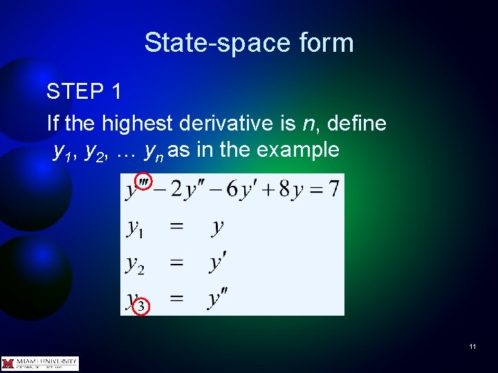
State-space form STEP 1 If the highest derivative is n, define y 1, y 2, … yn as in the example 11

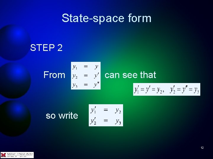
State-space form STEP 2 From can see that so write 12

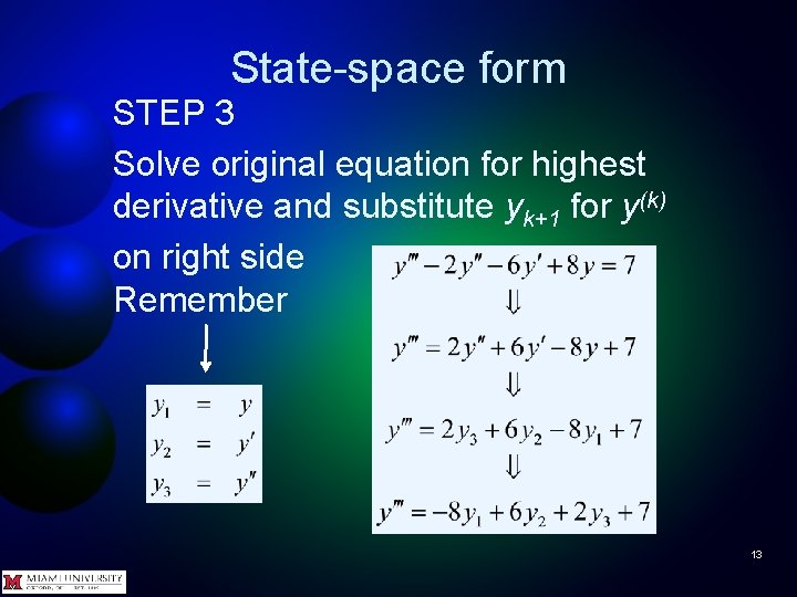
State-space form STEP 3 Solve original equation for highest derivative and substitute yk+1 for y(k) on right side Remember 13

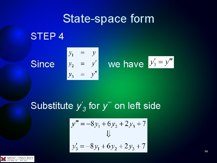
State-space form STEP 4 Since we have Substitute y'3 for y''' on left side 14

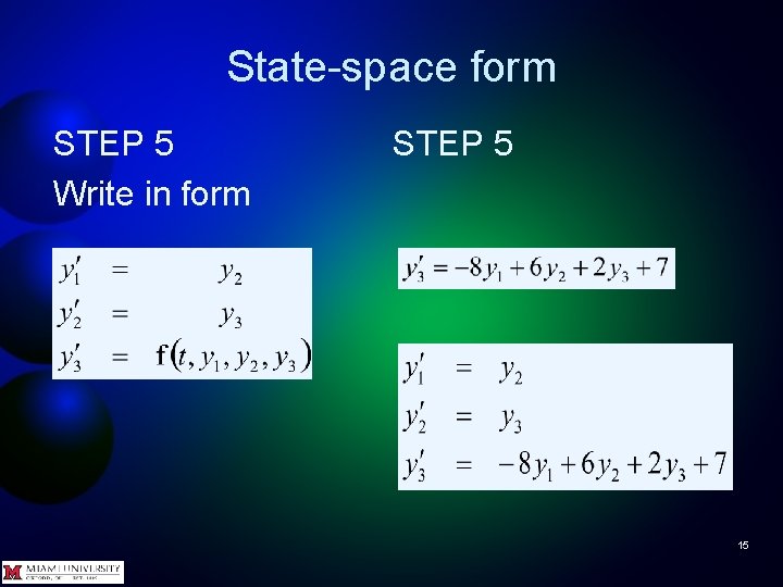
State-space form STEP 5 Write in form STEP 5 15

State-space form STEP 6 Write system of equations as MATLAB function that accepts a scalar (time) and one column vector (y-values at the given time) and returns one column vector (y'-values at the given time). 16

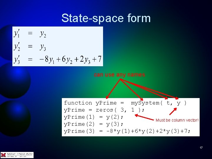
State-space form can use any names function y. Prime = my. System( t, y ) y. Prime = zeros( 3, 1 ); y. Prime(1) = y(2); Must be column vector! y. Prime(2) = y(3); y. Prime(3) = -8*y(1)+6*y(2)+2*y(3)+7; 17

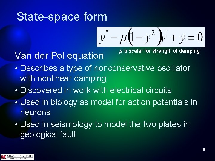
State-space form Van der Pol equation μ is scalar for strength of damping • Describes a type of nonconservative oscillator with nonlinear damping • Discovered in work with electrical circuits • Used in biology as model for action potentials in neurons • Used in seismology to model the two plates in geological fault 18

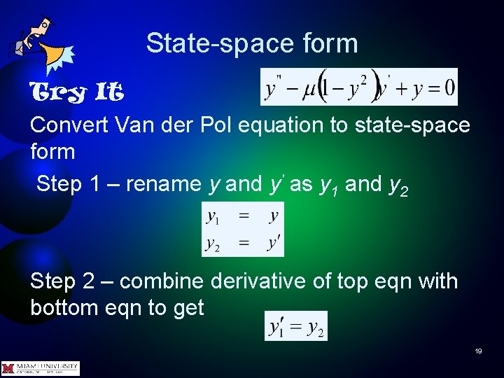
State-space form Try It Convert Van der Pol equation to state-space form Step 1 – rename y and y' as y 1 and y 2 Step 2 – combine derivative of top eqn with bottom eqn to get 19

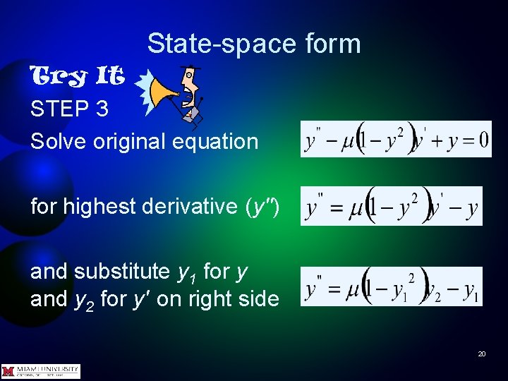
State-space form Try It STEP 3 Solve original equation for highest derivative (y'') and substitute y 1 for y and y 2 for y' on right side 20

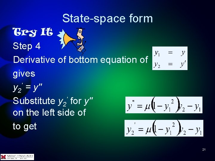
State-space form Try It Step 4 Derivative of bottom equation of gives y 2' = y'' Substitute y 2' for y'' on the left side of to get 21

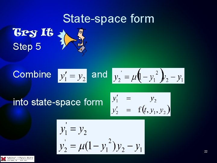
State-space form Try It Step 5 Combine and into state-space form 22

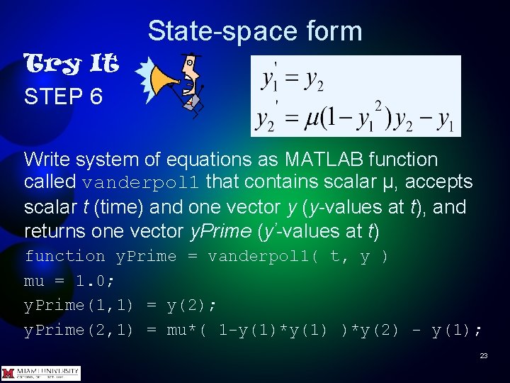
State-space form Try It STEP 6 Write system of equations as MATLAB function called vanderpol 1 that contains scalar μ, accepts scalar t (time) and one vector y (y-values at t), and returns one vector y. Prime (y’-values at t) function y. Prime = vanderpol 1( t, y ) mu = 1. 0; y. Prime(1, 1) = y(2); y. Prime(2, 1) = mu*( 1 -y(1)*y(1) )*y(2) - y(1); 23

State-space form Try It STEP 7 Ta-dah! Ready to solve. Well, almost. . . PROBLEM In general, there are many functions that satisfy a given ODE. Need additional information to get specific solution. 24

State-space form Questions? 25

Initial value problem Two common ways to specify the extra information needed to produce only one solution of differential equation. Let's start with one way. It's called the Initial Value Problem 26

Initial value problem In initial value problem, solution of interest satisfies a specific initial condition, i. e. , y = y 0 at initial time t 0 For state-space form, initial value problem is y' = f(t, y) and y(t 0) = y 0 If f(t, y) is "sufficiently smooth", problem has exactly one solution. Generally, no analytic expression so must solve numerically 27

Initial value problem Some kind of differential equations are stiff problems. Will discuss stiffness later. Right now, let's work on nonstiff problems 28

Initial value problem MATLAB has three solvers for nonstiff equations ode 45 – A one-step solver – in computing , needs only solution at immediately preceding time point – Best function to apply as a "first try" for most problems. ode 23 – A one-step solver – May be more efficient than ode 45() at crude tolerances and in presence of mild stiffness ode 113 – A multistep solver – needs solutions at several preceding time points to compute current solution – May be more efficient than ode 45() at stringent tolerances and when ODE function is particularly expensive to evaluate 29

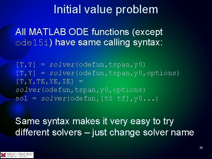
Initial value problem All MATLAB ODE functions (except ode 15 i) have same calling syntax: [T, Y] = solver(odefun, tspan, y 0) [T, Y] = solver(odefun, tspan, y 0, options) [T, Y, TE, YE, IE] = solver(odefun, tspan, y 0, options) sol = solver(odefun, [t 0 tf], y 0. . . ) Same syntax makes it very easy to try different solvers – just change solver name 30

Initial value problem [T, Y] = solver(odefun, tspan, y 0) [T, Y] = solver(odefun, tspan, y 0, options) • odefun – a function handle that evaluates the right side of the differential equations • tspan – a vector specifying the interval of integration, [t 0, tf]. The solver imposes the initial conditions at tspan(1), and integrates from tspan(1) to tspan(2) • y 0 – A vector of initial conditions • options – Structure of optional parameters that change the default integration 31

Initial value problem Outputs of ODE solvers [T, Y] = solver(odefun, tspan, y 0) [T, Y] = solver(odefun, tspan, y 0, options) [T, Y, TE, YE, IE] = solver(odefun, tspan, y 0, options) T – column vector of time points Y – solution array – One row is solution of all elements of y at time given in T in same row – One column is solution of one element of y for all times in T – Y(m, n) is value of yn at time tm Will look at other outputs later 32

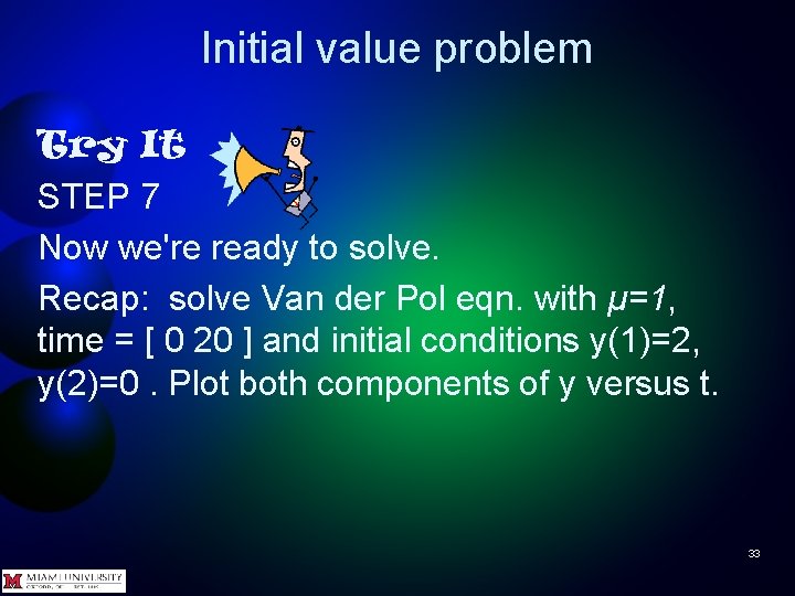
Initial value problem Try It STEP 7 Now we're ready to solve. Recap: solve Van der Pol eqn. with μ=1, time = [ 0 20 ] and initial conditions y(1)=2, y(2)=0. Plot both components of y versus t. 33

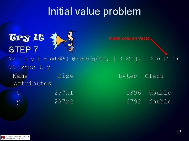
Initial value problem Try It STEP 7 make column vector >> [ t y ] = ode 45( @vanderpol 1, [ 0 20 ], [ 2 0 ]' ); >> whos t y Name Size Attributes t 237 x 1 y 237 x 2 Bytes 1896 3792 Class double 34

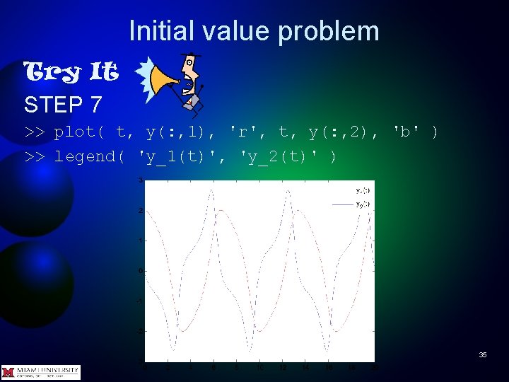
Initial value problem Try It STEP 7 >> plot( t, y(: , 1), 'r', t, y(: , 2), 'b' ) >> legend( 'y_1(t)', 'y_2(t)' ) 35

Initial value problem Try It Rewrite vanderpol 1. m as vanderpol 2. m. Make the new version of the function accept μ as the third argument. Run vanderpol 2 as an anonymous function, using the same initial conditions and value of μ as before. 36

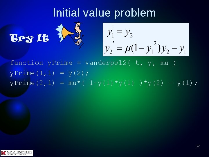
Initial value problem Try It function y. Prime = vanderpol 2( t, y, mu ) y. Prime(1, 1) = y(2); y. Prime(2, 1) = mu*( 1 -y(1)*y(1) )*y(2) - y(1); 37

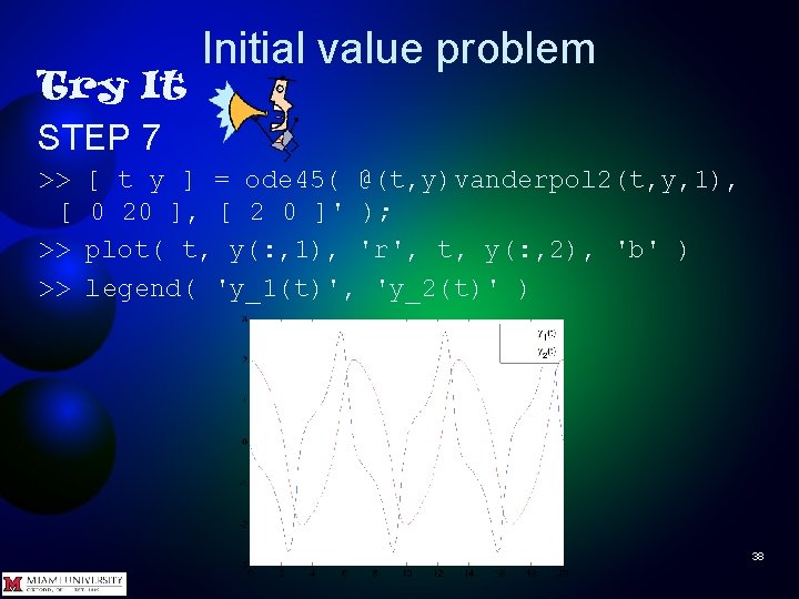
Try It STEP 7 >> [ >> >> Initial value problem [ t y ] = ode 45( @(t, y)vanderpol 2(t, y, 1), 0 20 ], [ 2 0 ]' ); plot( t, y(: , 1), 'r', t, y(: , 2), 'b' ) legend( 'y_1(t)', 'y_2(t)' ) 38

Initial value problem Try It Let's try another initial value problem – a mass on a spring. 39

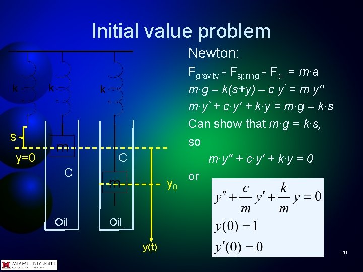
Initial value problem Newton: k s y=0 k k m C Oil C m y 0 Fgravity - Fspring - Foil = m∙a m∙g – k(s+y) – c y' = m y'' m∙y'' + c∙y' + k∙y = m∙g – k∙s Can show that m∙g = k∙s, so m∙y'' + c∙y' + k∙y = 0 or Oil y(t) 40

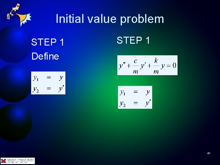
Initial value problem STEP 1 Define STEP 1 41

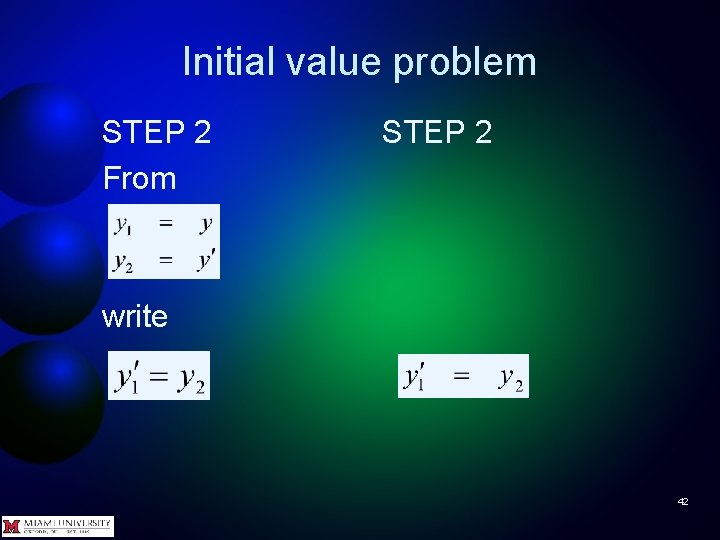
Initial value problem STEP 2 From STEP 2 write 42

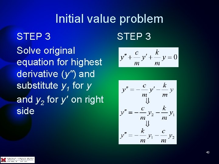
Initial value problem STEP 3 Solve original equation for highest derivative (y'') and substitute y 1 for y and y 2 for y' on right side STEP 3 43

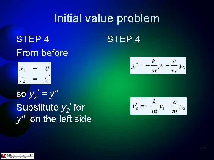
Initial value problem STEP 4 From before STEP 4 so y 2' = y'' Substitute y 2' for y'' on the left side 44

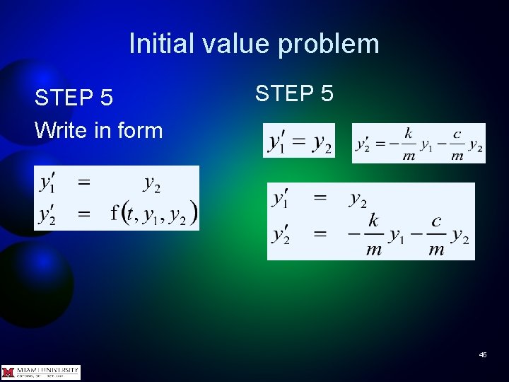
Initial value problem STEP 5 Write in form STEP 5 45

Initial value problem STEP 6 Write system of equations as MATLAB function that accepts a scalar t (time) and one vector (y-values at t) and returns one vector (y’-values at t), as shown on next slide 46

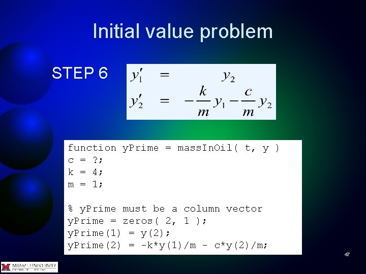
Initial value problem STEP 6 function y. Prime = mass. In. Oil( t, y ) c = ? ; k = 4; m = 1; % y. Prime must be a column vector y. Prime = zeros( 2, 1 ); y. Prime(1) = y(2); y. Prime(2) = -k*y(1)/m - c*y(2)/m; 47

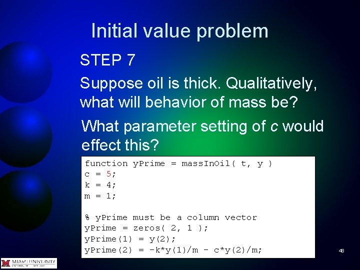
Initial value problem STEP 7 Suppose oil is thick. Qualitatively, what will behavior of mass be? What parameter setting of c would effect this? function y. Prime = mass. In. Oil( t, y ) c = 5; ? ; k = 4; m = 1; % y. Prime must be a column vector y. Prime = zeros( 2, 1 ); y. Prime(1) = y(2); y. Prime(2) = -k*y(1)/m - c*y(2)/m; 48

Initial value problem STEP 7 c=5 Solution for first 10 seconds >> [t y] = ode 45( @mass. In. Oil, [0 10], [1 0] ); >> plot(t, y(: , 1)) y(0) = 1 y'(0) = 0 49

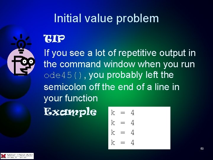
Initial value problem TIP If you see a lot of repetitive output in the command window when you run ode 45(), you probably left the semicolon off the end of a line in your function Example k = 4 50

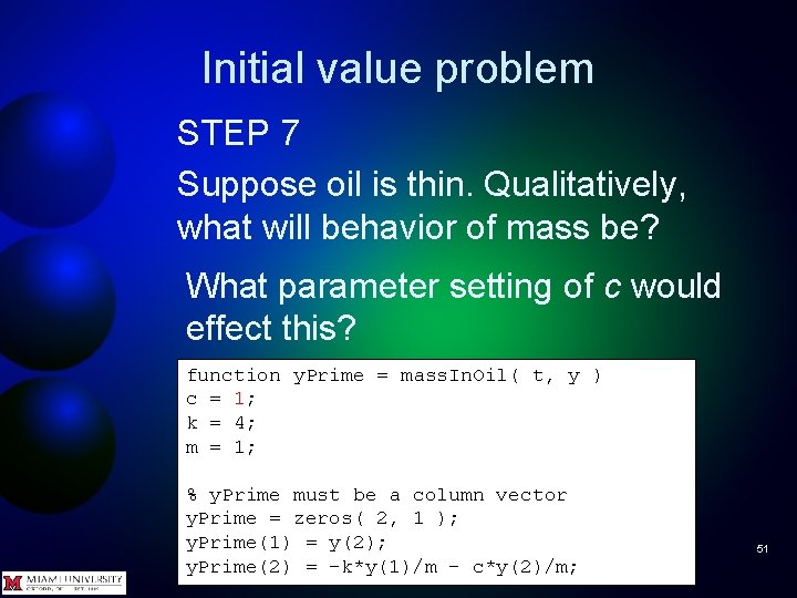
Initial value problem STEP 7 Suppose oil is thin. Qualitatively, what will behavior of mass be? What parameter setting of c would effect this? function y. Prime = mass. In. Oil( t, y ) c = 1; ? ; k = 4; m = 1; % y. Prime must be a column vector y. Prime = zeros( 2, 1 ); y. Prime(1) = y(2); y. Prime(2) = -k*y(1)/m - c*y(2)/m; 51

Initial value problem STEP 7 c=1 >> [t y] = ode 45( @mass. In. Oil, [0 10], [1 0] ); >> plot(t, y(: , 1)) 52

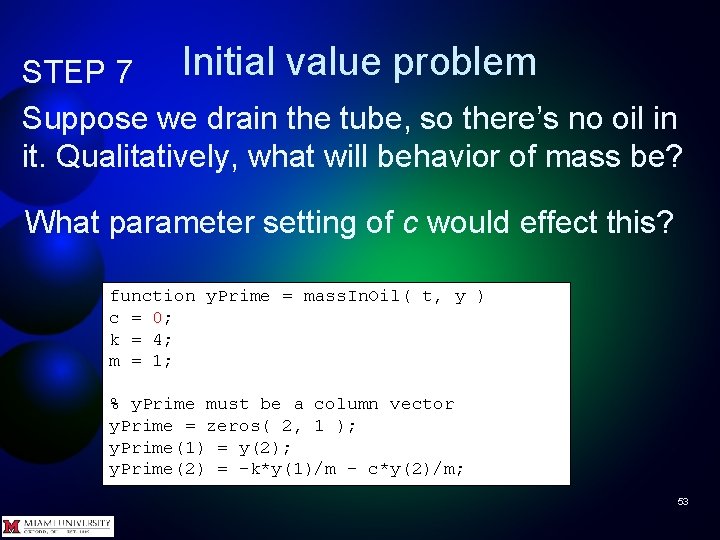
Initial value problem STEP 7 Suppose we drain the tube, so there’s no oil in it. Qualitatively, what will behavior of mass be? What parameter setting of c would effect this? function y. Prime = mass. In. Oil( t, y ) c = 0; ? ; k = 4; m = 1; % y. Prime must be a column vector y. Prime = zeros( 2, 1 ); y. Prime(1) = y(2); y. Prime(2) = -k*y(1)/m - c*y(2)/m; 53

Initial value problem STEP 7 c=0 >> [t y] = ode 45( @mass. In. Oil, [0 10], [1 0] ); >> plot(t, y(: , 1)) 54

Initial value problems Questions so far? 55

Stiff equations "Stiffness is a subtle, difficult, and important concept in the numerical solution of ordinary differential equations. " - Cleve Moler, inventor of MATLAB 56

Stiff equations Three definitions of stiffness • A problem is stiff if the solution being sought varies slowly, but there are nearby solutions that vary rapidly, so the numerical method must take small steps to obtain satisfactory results. • A property of some differential equations in which some states change very rapidly while others may change very slowly. • For a stiff problem, solutions can change on a time scale that is very short compared to the interval of integration, but the solution of interest changes on a much longer time scale. 57

Stiff equations Stiffness • Depends on the differential equation, initial conditions, and numerical solution method • Stiffness is an efficiency issue – If you don't care how much computation time a problem takes, you don't need to worry about stiffness – Nonstiff numerical methods can solve stiff problems – they just take a long time to do it 58

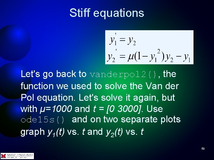
Stiff equations Let's go back to vanderpol 2(), the function we used to solve the Van der Pol equation. Let's solve it again, but with μ=1000 and t = [0 3000]. Use ode 15 s() and on two separate plots graph y 1(t) vs. t and y 2(t) vs. t 59

Stiff equations Try It >> [ t y ] = ode 15 s(. . . @(t, y)vanderpol 2(t, y, 1000), [0 3000], [2 0]'); >> plot( t, y(: , 1) ) >> title( 'y_1(t) vs. t' ) >> figure >> plot( t, y(: , 2) ) >> title( 'y_2(t) vs. t' ) 60

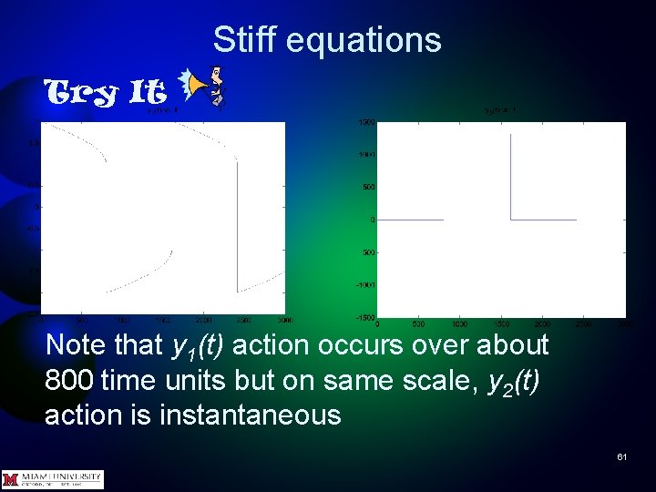
Stiff equations Try It Note that y 1(t) action occurs over about 800 time units but on same scale, y 2(t) action is instantaneous 61

Stiff equations Can find out how much work a solver did [t y] = solver( fun, t. Span, y 0, options ) To make solver display processing statistics, set "Stats" to "on" in options by using function odeset() For more options, type help odeset 62

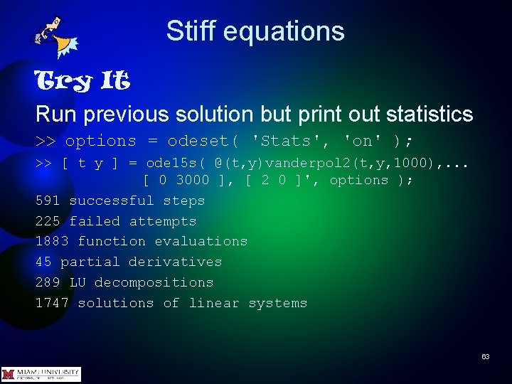
Stiff equations Try It Run previous solution but print out statistics >> options = odeset( 'Stats', 'on' ); >> [ t y ] = ode 15 s( @(t, y)vanderpol 2(t, y, 1000), . . . [ 0 3000 ], [ 2 0 ]', options ); 591 successful steps 225 failed attempts 1883 function evaluations 45 partial derivatives 289 LU decompositions 1747 solutions of linear systems 63

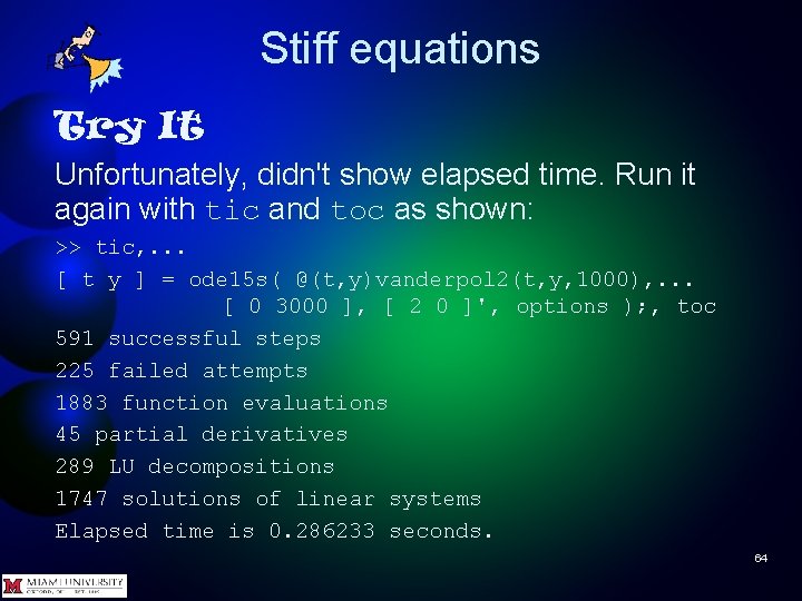
Stiff equations Try It Unfortunately, didn't show elapsed time. Run it again with tic and toc as shown: >> tic, . . . [ t y ] = ode 15 s( @(t, y)vanderpol 2(t, y, 1000), . . . [ 0 3000 ], [ 2 0 ]', options ); , toc 591 successful steps 225 failed attempts 1883 function evaluations 45 partial derivatives 289 LU decompositions 1747 solutions of linear systems Elapsed time is 0. 286233 seconds. 64

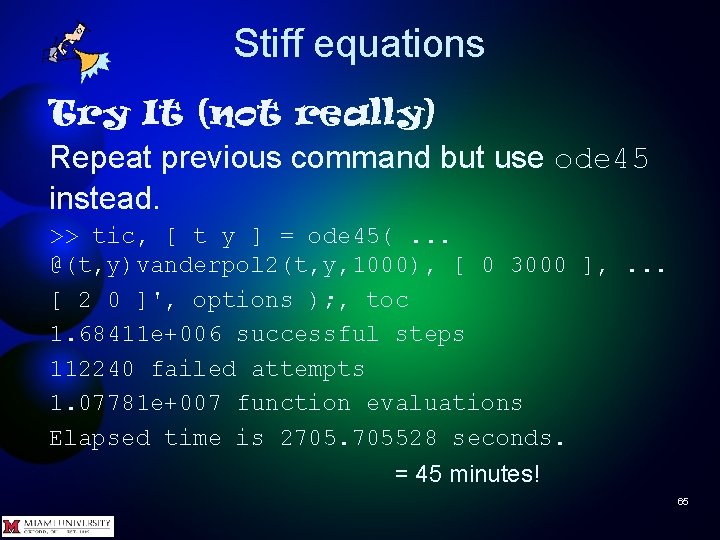
Stiff equations Try It (not really) Repeat previous command but use ode 45 instead. >> tic, [ t y ] = ode 45(. . . @(t, y)vanderpol 2(t, y, 1000), [ 0 3000 ], . . . [ 2 0 ]', options ); , toc 1. 68411 e+006 successful steps 112240 failed attempts 1. 07781 e+007 function evaluations Elapsed time is 2705. 705528 seconds. = 45 minutes! 65

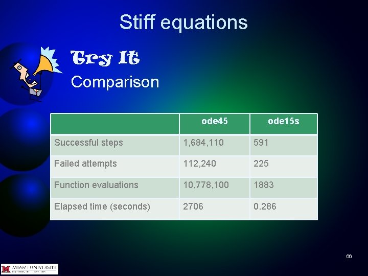
Stiff equations Try It Comparison ode 45 ode 15 s Successful steps 1, 684, 110 591 Failed attempts 112, 240 225 Function evaluations 10, 778, 100 1883 Elapsed time (seconds) 2706 0. 286 66

Stiff equations Questions? 67

Linearly implicit equations Up to now have only dealt with equations that can be put into statespace form. Another kind of equation is the linearly implicit ODE: M(t, y)y' = f(t, y) where M(t, y) is a matrix. This is a generalization of state-space formulation 68

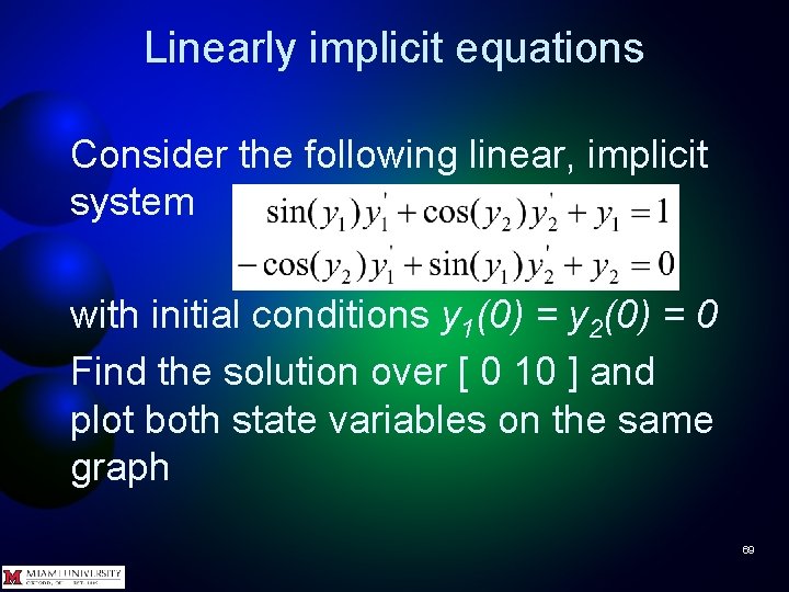
Linearly implicit equations Consider the following linear, implicit system with initial conditions y 1(0) = y 2(0) = 0 Find the solution over [ 0 10 ] and plot both state variables on the same graph 69

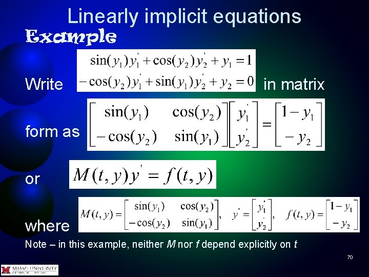
Linearly implicit equations Example Write in matrix form as or where Note – in this example, neither M nor f depend explicitly on t 70

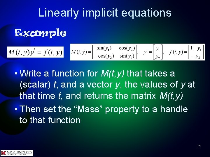
Linearly implicit equations Example • Write a function for M(t, y) that takes a (scalar) t, and a vector y, the values of y at that time t, and returns the matrix M(t, y) • Then set the “Mass” property to a handle to that function 71

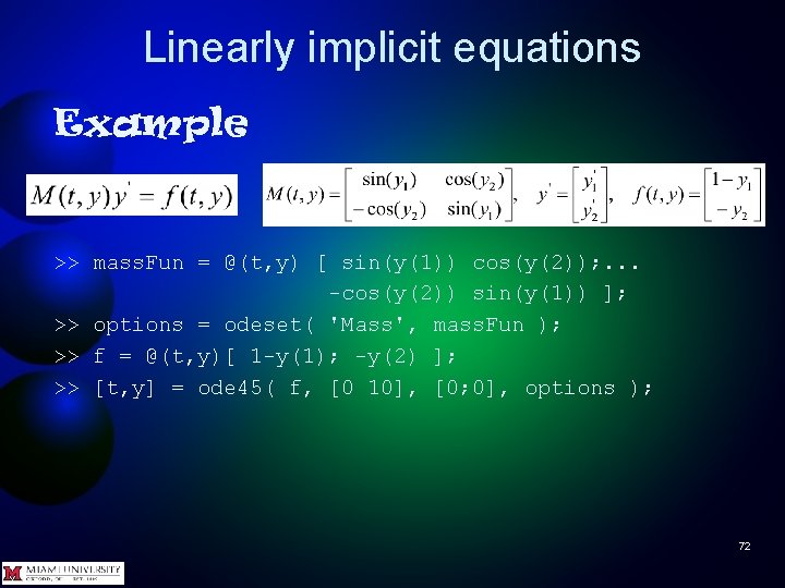
Linearly implicit equations Example >> mass. Fun = @(t, y) [ sin(y(1)) cos(y(2)); . . . -cos(y(2)) sin(y(1)) ]; >> options = odeset( 'Mass', mass. Fun ); >> f = @(t, y)[ 1 -y(1); -y(2) ]; >> [t, y] = ode 45( f, [0 10], [0; 0], options ); 72

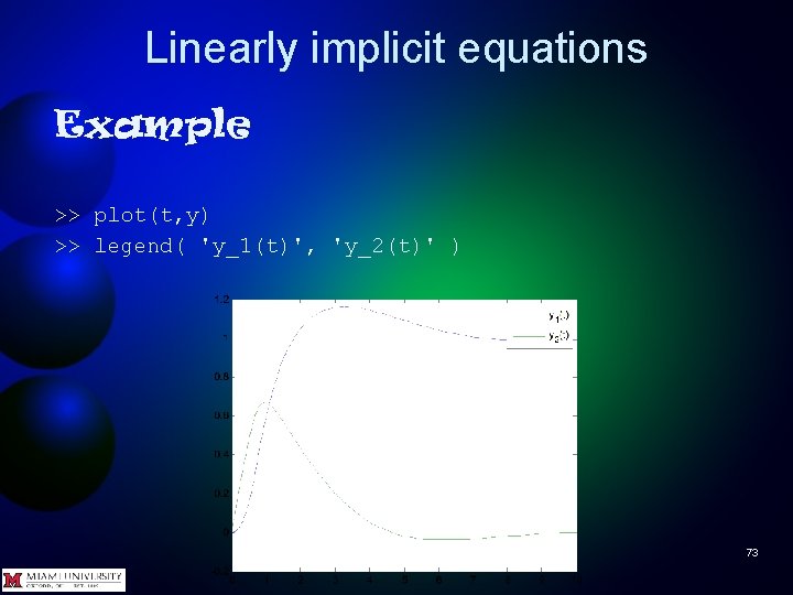
Linearly implicit equations Example >> plot(t, y) >> legend( 'y_1(t)', 'y_2(t)' ) 73

Linearly implicit equations Questions? 74

Events Usually run a simulation from a start time to a stop time. Sometimes would rather stop when something happens than when solver reaches a certain time. For example • Equations no longer valid at event – Force of gravity between two bodies varies inversely as square of distance. As two bodies get very close, force becomes infinite 75

Events • No longer interested in solution – If computing fall of parachutist, none but the sickest among us cares what happens after she hits the ground • Only want to see a few cycles of a periodic solution 76

Events MATLAB's ODE solvers have a facility for detecting and acting on events. You create a function and pass a handle to it as part of the options passed to the solver. The solver will then give you information about any events that occur and act on them, e. g. , stop solving. 77

Events The function's form is [value, isterminal, direction] = events(t, y) value, isterminal, and direction are vectors for which the ith element corresponds to the ith event • value(i) is the value of the ith event function. Want to make it zero • isterminal(i) = 1 if the integration is to terminate at a zero of this event function, otherwise, 0 78

Events [value, isterminal, direction] = events(t, y) • direction(i) = 0 if all zeros are to be located (the default), +1 if only zeros where the event function is increasing, and -1 if only zeros where the event function is decreasing 79

Events If you specify an events function call the solver as [T, Y, TE, YE, IE] =. . . solver(odefun, tspan, y 0, options) The three additional outputs are: • TE - column vector of times at which events occur • YE - solution values corresponding to these times • IE - indexes into the vector returned by the events function. The values indicate which event the solver detected. If no events detected, TE, YE, IE will be empty 80

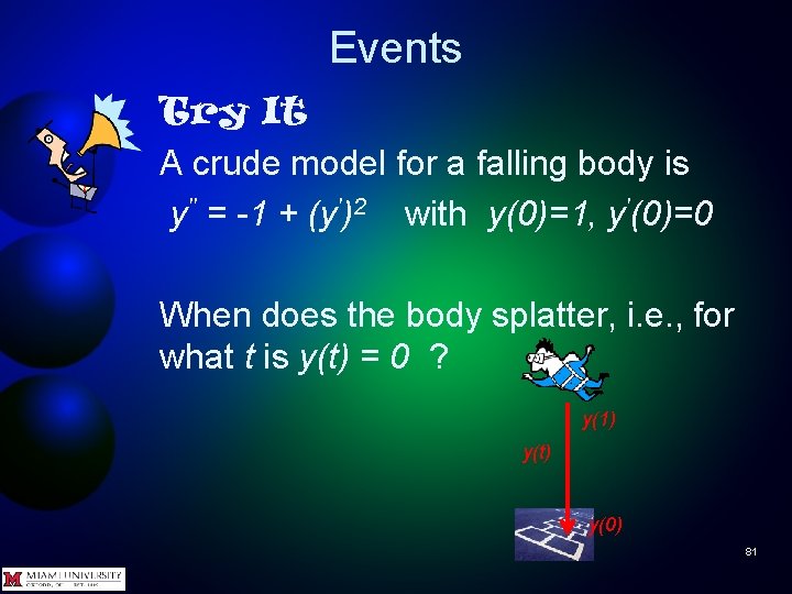
Events Try It A crude model for a falling body is y'' = -1 + (y')2 with y(0)=1, y'(0)=0 When does the body splatter, i. e. , for what t is y(t) = 0 ? y(1) y(t) y(0) 81

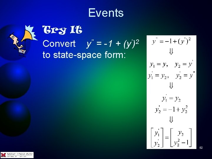
Events Try It Convert y'' = -1 + (y')2 to state-space form: 82

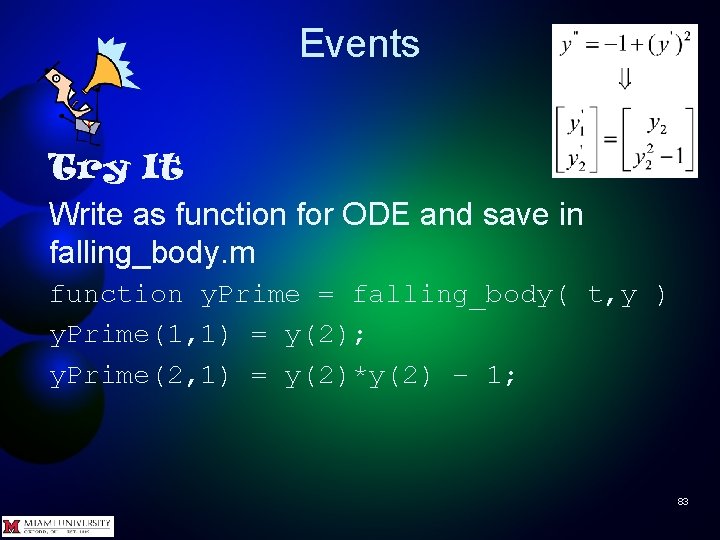
Events Try It Write as function for ODE and save in falling_body. m function y. Prime = falling_body( t, y ) y. Prime(1, 1) = y(2); y. Prime(2, 1) = y(2)*y(2) – 1; 83

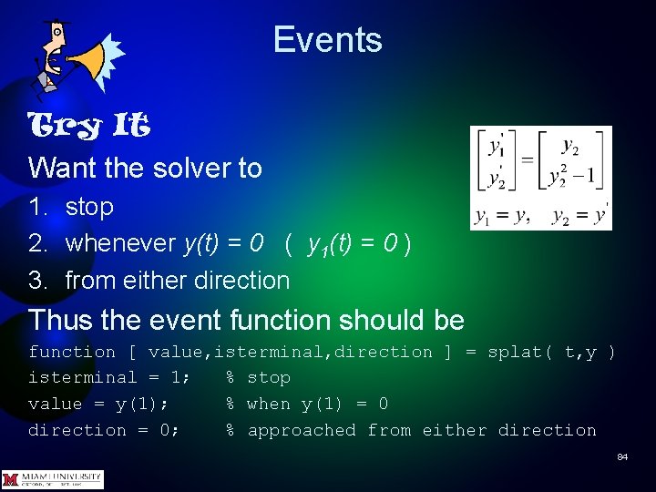
Events Try It Want the solver to 1. stop 2. whenever y(t) = 0 ( y 1(t) = 0 ) 3. from either direction Thus the event function should be function [ value, isterminal, direction ] = splat( t, y ) isterminal = 1; % stop value = y(1); % when y(1) = 0 direction = 0; % approached from either direction 84

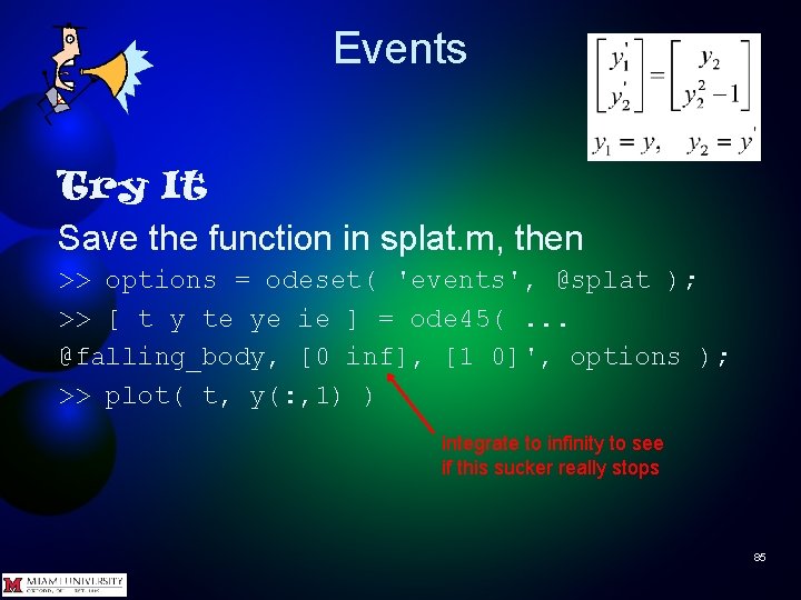
Events Try It Save the function in splat. m, then >> options = odeset( 'events', @splat ); >> [ t y te ye ie ] = ode 45(. . . @falling_body, [0 inf], [1 0]', options ); >> plot( t, y(: , 1) ) integrate to infinity to see if this sucker really stops 85

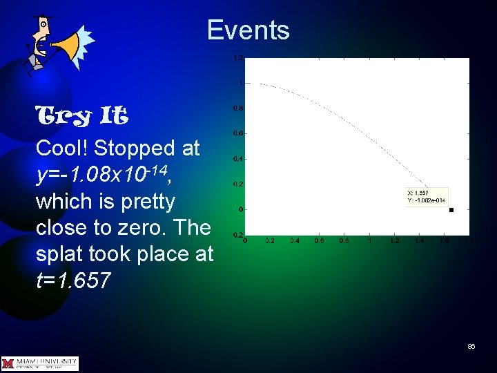
Events Try It Cool! Stopped at y=-1. 08 x 10 -14, which is pretty close to zero. The splat took place at t=1. 657 86

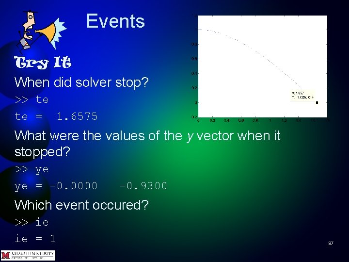
Events Try It When did solver stop? >> te te = 1. 6575 What were the values of the y vector when it stopped? >> ye ye = -0. 0000 -0. 9300 Which event occured? >> ie ie = 1 87

Multiple Events Try It Let’s also make a note (but not stop solving) of when the parachutist’s heart rate goes above 200 beats per minute (bpm) 1. Don’t stop 2. Whenever heart-beat rate goes above 200 bpm 3. In increasing direction (goes above) 88

Multiple Events Try It Assume heart beats given by heartbeats(t) = 100 + 100*t Save a copy of splat. m as splat 2. m and rewrite as 89

Multiple Events Try It function [ value, isterminal, direction ] = splat 2( t, y ) % first event isterminal(1) = 1; value(1) = y(1); direction(1) = 0; % stop % when y(1) = 0 % approached from either direction % second event isterminal(2) = 0; % don't stop heart. Beats = 100 + 100 * t; % beats per minute (bpm) value(2) = heart. Beats - 200; % bpm over or under 200 % only trigger when value(2) crosses zero while increasing direction(2) = +1; 90

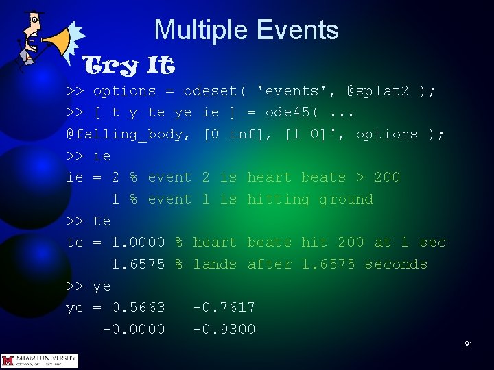
Multiple Events Try It >> options = odeset( 'events', @splat 2 ); >> [ t y te ye ie ] = ode 45(. . . @falling_body, [0 inf], [1 0]', options ); >> ie ie = 2 % event 2 is heart beats > 200 1 % event 1 is hitting ground >> te te = 1. 0000 % heart beats hit 200 at 1 sec 1. 6575 % lands after 1. 6575 seconds >> ye ye = 0. 5663 -0. 7617 -0. 0000 -0. 9300 91

Events Questions? 92

The End 93

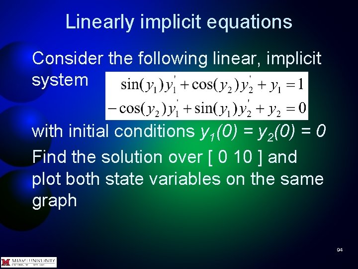
Linearly implicit equations Consider the following linear, implicit system with initial conditions y 1(0) = y 2(0) = 0 Find the solution over [ 0 10 ] and plot both state variables on the same graph 94

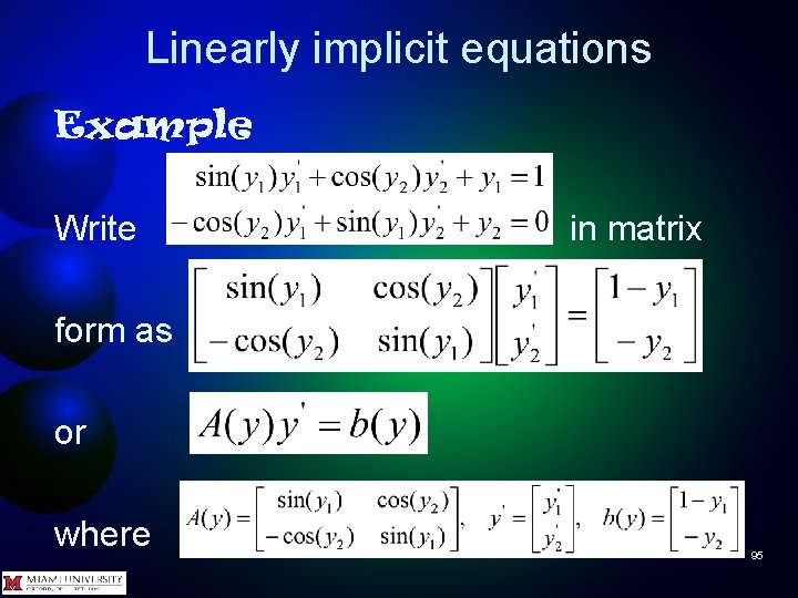
Linearly implicit equations Example Write in matrix form as or where 95

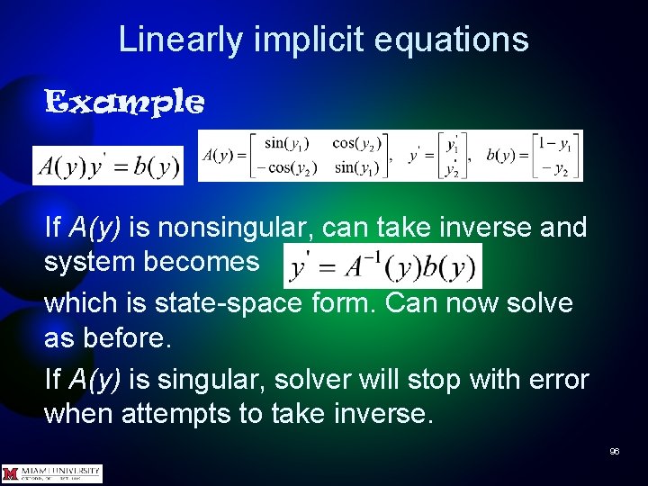
Linearly implicit equations Example If A(y) is nonsingular, can take inverse and system becomes which is state-space form. Can now solve as before. If A(y) is singular, solver will stop with error when attempts to take inverse. 96

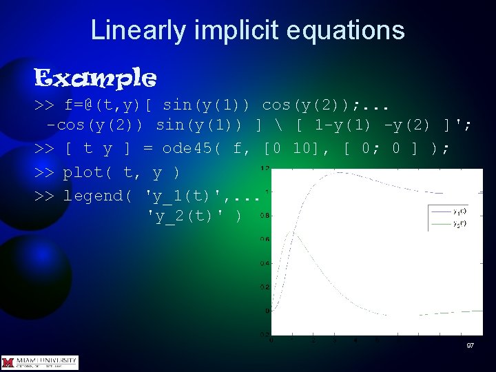
Linearly implicit equations Example >> f=@(t, y)[ sin(y(1)) cos(y(2)); . . . -cos(y(2)) sin(y(1)) ] [ 1 -y(1) -y(2) ]'; >> [ t y ] = ode 45( f, [0 10], [ 0; 0 ] ); >> plot( t, y ) >> legend( 'y_1(t)', . . . 'y_2(t)' ) 97