MATLAB MATLAB and Its Engineering Application EMail huzfcqupt

MATLAB及其 程应用 MATLAB and It’s Engineering Application 主讲教师： 胡章芳 E-Mail: huzf@cqupt. edu. cn

Chapter 2 MATLAB Basics • • • • 2. 1 Variables and Arrays 2. 2 Initializing Variables in MATLAB 2. 3 Multidimensional Arrays 2. 4 Subarrays 2. 5 Special Values 2. 6 Displaying Output Data 2. 7 Data Files 2. 8 Scalar and Array Operations All sections about 2. 9 Hierarchy of Operations Plotting will be 2. 10 Built-in MATLAB Functions introduced in a separated chapter. 2. 11 Introduction to Plotting 2. 12 Examples 2. 13 Debugging MATLAB Programs 2. 14 Summary

Introduction In this chapter, we will introduce more basic elements of the MATLAB language. By the end of the chapter, you will be able to write simple but functional MATLAB programs.

Review l. A program can be input v. Typing commands using the command line (lines starting with “» ” on the MATLAB desktop) v. As a series of commands using a file (a special file called M-file) l If a command is followed by a semicolon (; ), result of the computation is not shown on the command window

2. 1 Variables and Arrays l. The fundamental unit of data is array An array is a collection of data values organized into rows and columns. scalar value 3 1 40 -3 11 15 -2 3 21 -4 1 0 13 vector matrix

2. 1 Variables and Arrays v. Data values within an array are accessed by including the name of the array followed by subscripts in parentheses. array arr Row 1 The shaded element in this array would be addressed as Row 2 arr(3, 2). Row 3 Row 4 Col 1 Col 2 Col 3 Col 4 Col 5

A(2, 1) = 3, and C(2) = 2

2. 1 Variables and Arrays • Arrays can be classified as either vectors or matrices. • The term “vector” is usually used to describe an array with only one dimension; • The term “matrix” is usually used to describe an array with two or more dimensions. • The size of an array:

2. 1 Variables and Arrays l. Variable is a name given to a reserved location in memory class_code = 111; number_of_students = 65; name = ‘Chongqing University of Posts and Telecommunications'; radius = 5; area = pi * radius^2;

2. 1 Variables and Arrays l MATLAB variable names vmust begin with a letter vcan contain any combination of letters, numbers and underscore (_) vmust be unique in the first 31 characters l MATLAB is case sensitive “name”, “Name” and “NAME” are considered different variables l Never use a variable with the same name as a MATLAB command l Naming convention: use lowercase letters

2. 1 Variables and Arrays l Use meaningful names for variables l number_of_students l exchange_rate

2. 1 Variables and Arrays • data dictionary: • The most common types of MATLAB variables are double and char: • Double: consist of scalars or array of 64 -bit double-precision floating-point numbers. 10 -308~10308 • Char: consist of scalars or array of 16 -bit values.

2. 1 Variables and Arrays • MATLAB: weakly typed language • C: strongly typed language

2. 2 Initializing Variables l. Three common ways: 1. Initialization using assignment statements; 2. Input data from the keyboard; 3. Read data from a file.

2. 2 Initializing Variables l 2. 2. 1 Initialization using assignment statements v. General form: var = expression x=5 x= 5 y=x+1 y= 6 vector = [ 1 2 3 4 ] vector = 1 2 3 4

2. 2 Initializing Variables matrix = [ 1 2 3; 4 5 6 ] matrix = 1 2 3 4 5 6 matrix = [ 1 2 3; 4 5 ] ? ? ? Error a = [ 5 (2+4) ] a= 5 6

2. 2 Initializing Variables • 2. 2. 2 Initialization using shortcut statements vcolon operator first: increment: last x = 1: 2: 10 x= 1 3 5 7 9 y = 0: 0. 1: 0. 5 y= 0 0. 1 0. 2 0. 3 0. 4 0. 5

2. 2 Initializing Variables l. Transpose operator ' u = [ 1: 3 ]' u= 1 2 3 v=[uu] v= 1 1 2 2 3 3 v = [ u'; u' ] v= 1 2 3

2. 2 Initializing Variables 2. 2. 3 Initialization using built-in functions vzeros() x = zeros(2) x= 0 0 y = zeros(1, 4) y= 0 0 0 z = zeros(2, 3) z= 0 0 0 vones(), size(), length() t = zeros( size(z) ) t= 0 0 0 0

2. 2 Initializing Variables 2. 2. 4 Initialization using keyboard input vinput() value = input( 'Enter an value: ' ) Enter an value: 1. 25 value = 1. 2500 name = input( 'What is your name: ', 's' ) What is your name: Selim name = Selim

2. 3 Multidimensional Arrays l. Initialization c(: , 1)=[1 2 3; 4 5 6]; c(: , 2)=[7 8 9; 10 11 12]; whos Name Size c 2 x 3 x 2 c c(: , 1) = 1 2 3 4 5 6 c(: , 2) = 7 8 9 10 11 12 Bytes Class 96 double array

2. 3 Multidimensional Arrays l Storing in Memory v. Two-dimensional : Column major order v. Multidimensional Arrays : array subscript incremented first, second, third, … (1, 1, 1), (2, 1, 1), (1, 2, 1), (2, 2, 1), (1, 1, 2), (2, 1, 2), (1, 2, 2), (2, 2, 2) l Accessing Multidimensional arrays with a Single Subscript v. The elements will be accessed in the order in which they were allocated in memory c(5)

2. 4 Subarrays l. Array indices start from 1 x = [ -2 0 9 1 4 ]; x(2) ans = 0 x(4) ans = 1 x(8) ? ? ? Error x(-1) ? ? ? Error

2. 4 Subarrays y = [ 1 2 3; 4 5 6 ]; y(1, 2) ans = 2 y(2, 1) ans = 4 y(2) ans = 4 y(1, 1) 1 y(1) y(2, 1) 4 y(2) y(1, 2) 2 y(3) y(2, 2) 5 y(4) y(1, 3) 3 y(5) y(2, 3) 6 y(6) (column major order)

2. 4 Subarrays y = [ 1 2 3; 4 5 6 ]; y(1, : ) ans = 1 2 y(: , 2) ans = 2 5 y(2, 1: 2) ans = 4 5 3 y(1, 2: end) ans = 2 3 y(: , 2: end) ans = 2 3 5 6

2. 4 Subarrays x = [ -2 0 9 1 4 ]; x(2) = 5 x= -2 5 9 x(4) = x(1) x= -2 5 9 x(8) = -1 x= -2 5 9 1 4 -2 4 0 0 -1

2. 4 Subarrays y = [ 1 2 3; 4 5 6 ]; y(1, 2) = -5 y= 1 4 -5 5 3 6 y(2, 1) = 0 y= 1 0 -5 5 3 6 y(1, 2: end) = [ -1 9 ] y= 1 0 -1 5 9 6

2. 4 Subarrays y = [ 1 2 3; 4 5 6; 7 8 9 ]; y(2: end, 2: end) = 0 y= 1 4 7 2 0 0 3 0 0 y(2: end, 2: end) = [ -1 5 ] ? ? ? Error y(2, [1 3]) = -2 y= 1 -2 7 2 0 0 3 -2 0

2. 5 Special Values v pi: value up to 15 significant digits v i, j: sqrt(-1) v Inf: infinity (such as division by 0) v Na. N: Not-a-Number (such as division of zero by zero) v clock: current date and time as a vector v date: current date as a string (e. g. 20 -Feb-2008) v eps: epsilon v ans: default variable for answers

2. 6 Displaying Output Data l 2. 6. 1 Changing the data format value = 12. 345678901234567 format short 12. 3457 long 12. 34567890123457 short e 1. 2346 e+001 long e 1. 234567890123457 e+001 rat 1000/81 compact loose

2. 6 Displaying Output Data l 2. 6. 2 The disp( array ) function disp( 'Hello' ); Hello disp(5); 5 disp( [ ‘重庆邮电大学’ ] ); 重庆邮电大学 name = 'Selim'; disp( [ 'Hello ' name ] ); Hello Selim

2. 6 Displaying Output Data 2. 6. 2 The num 2 str() and int 2 str() functions d = [ num 2 str(25) '-Feb-' num 2 str(2008) ]; disp(d); 25 -Feb-2008 x = 23. 11; disp( [ 'answer = ' num 2 str(x) ] ); answer = 23. 11 disp( [ 'answer = ' int 2 str(x) ] ); answer = 23

2. 6 Displaying Output Data 2. 6. 3 The fprintf( format, data ) function %d integer %f floating point format %e exponential format n skip to a new line g either floating point format or exponential format, whichever is shorter. Limitation: it only displays the real portion of a complex value.

2. 6 Displaying Output Data fprintf( 'Result is %d', 3 ); Result is 3 fprintf( 'Area of a circle with radius %d is %f', 3, pi*3^2 ); Area of a circle with radius 3 is 28. 274334 x = 5; fprintf( 'x = %3 d', x ); x= 5 x = pi; fprintf( 'x = %0. 2 f', x ); x = 3. 14 fprintf( 'x = %6. 2 f', x ); x = 3. 14 fprintf( 'x = %dny = %dn', 3, 13 ); x=3 y = 13

2. 7 Data Files vsave filename var 1 var 2 … save homework. mat x y binary Including: name, type, size, value But annot be read by other programs save x. dat x –ascii But name and type are lost; and the resulting data file will be much larger

2. 7 Data Files vload filename. mat binary load x. dat –ascii

2. 8 Scalar & Array Operations lvariable_name = expression; vaddition a+b vsubtraction a-b vmultiplication axb vdivision a/b vexponent ab a+b a-b a*b a/b a^b

2. 8. 1 Scalar & Array Operations l. Scalar-matrix operations a = [ 1 2; 3 4 ] a= 1 2 3 4 2*a ans = 2 4 6 8 a+4 ans = 5 6 7 8 l. Element-by-element operations a = [ 1 0; 2 1 ]; b = [ -1 2; 0 1 ]; a+b ans = 0 2 2 2 a. * b ans = -1 0 0 1

2. 8. 2 Array & Matrix Operations l. Matrix multiplication: C = A * B v. If ▪ A is a p-by-q matrix ▪ B is a q-by-r matrix then ▪ C will be a p-by-r matrix where

2. 8. 2 Array & Matrix Operations l. Matrix multiplication: C = A * B

2. 8. 2 Array & Matrix Operations l. Examples a = [ 1 2; 3 4 ] a= 1 2 3 4 b = [ -1 3; 2 -1 ] b= -1 3 2 -1 a. * b ans = -1 6 a*b ans = 3 5 6 -4 1 5

2. 8. 2 Array & Matrix Operations l. Examples a = [ 1 4 2; 5 7 3; 9 1 6 ] a= 1 4 2 5 7 3 9 1 6 b = [ 6 1; 2 5; 7 3 ] b= 6 1 2 5 7 3 c=a*b c= 28 27 65 49 98 32 d=b*a ? ? ? Error using ==> * Inner matrix dimensions must agree.

2. 8. 2 Array & Matrix Operations l. Identity matrix: I l. A * I = I * A = A l. Examples a = [ 1 4 2; 5 7 3; 9 1 6 ]; I = eye(3) I= 1 0 0 0 1 a*I ans = 1 4 2 5 7 3 9 1 6

2. 8. 2 Array & Matrix Operations l. Inverse of a matrix: A-1 l. AA-1 = A-1 A = I l. Examples a = [ 1 4 2; 5 7 3; 9 1 6 ]; b = inv(a) b= -0. 4382 0. 2472 0. 0225 0. 0337 0. 1348 -0. 0787 0. 6517 -0. 3933 0. 1461 a*b ans = 1. 0000 0 0 0. 0000 1. 0000 0 0 -0. 0000 1. 0000

2. 8. 2 Array & Matrix Operations l. Matrix left division: C = A B l. Used to solve the matrix equation AX = B where X = A-1 B l. In MATLAB, you can write x = inv(a) * b x=ab (second version is recommended)

2. 8. 2 Array & Matrix Operations l Example: Solving a system of linear equations A = [ 4 -2 6; 2 8 2; 6 10 3 ]; B = [ 8 4 0 ]'; X=AB X= -1. 8049 0. 2927 2. 6341

2. 8. 2 Array & Matrix Operations l. Matrix right division: C = A / B l. Used to solve the matrix equation XA = B where X = BA-1 l. In MATLAB, you can write x = b * inv(a) x=b/a (second version is recommended)

2. 9 Hierarchy of Operations v x=3*2+6/2 x=? l Processing order of operations is important ① parenthesis (starting from the innermost) ② exponentials (left to right) ③ multiplications and divisions (left to right) ④ additions and subtractions (left to right) x=3*2+6/2 x=9

2. 9 Hierarchy of Operations • Example p 49(2. 2) • You should always ask yourself: • will I easily understand this expression if I come back to it in six months? • Can another programmer look at my code and easily understand what I am doing? • Use extra parentheses • (2+4)/2

2. 10 Built-in Functions l General form: result = function_name( input ); vabs, sign vlog, log 10, log 2 vexp vsqrt vsin, cos, tan vasin, acos, atan vmax, min vround, floor, ceil, fix vmod, rem l help function_name

2. 10 Built-in Functions l Optional Results Can return more than one result. For example: [maxval index] = max ( [ 1 -5 6 -3 ] ) maxval = 6 index = 3 l Using MATLAB Function with Array Input v. You can call built-in functions with array inputs v. The function is applied to all elements of the array v. The result is an array with the same size as the input array

2. 10 Built-in Functions l Examples: x = [ 3 -2 9 4 -5 6 2 ]; abs(x) ans = 3 2 9 4 5 6 2 sin( [ 0 pi/6 pi/4 pi/3 pi/2 ] ) ans = 0 0. 5000 0. 7071 0. 8660 a = 1: 5; log(a) ans = 0 0. 6931 1. 0986 1. 3863 sqrt(-2) ans = 0 + 1. 4142 i 1. 0000 1. 6094

Example: 1. a=-3. 0, -2. 9, -2. 8, … 2. 8, 2. 9, 3. 0

U=[0. 89, 1. 20, 3. 09, 4. 27, 7. 71, 8. 99, 7. 92, 9. 70, 10. 41] i=[0. 028, 0. 040, 0. 100, 0. 145, 0. 118, 0. 258, 0. 299, 0. 257, 0. 308, 0. 345]

2. 11 Introduction to Plotting MATLAB’s extensive, device-independent plotting capabilities are one of its most powerful features. For example: x=0: 1: 10; y=x. ^2 -10. *x+15; Plot(x, y)

2. 11. 1 Using Simple xy Plots • • Functions: title xlabel and ylabel grid on and grid off For example: x=0: 1: 10; y=x. ^2 -10. *x+15; plot(x, y); title(‘plot of y=x. ^2 -10. *x+15’) xlabel(‘x’) ylabel(‘y’) grid on

2. 11. 2 Printing a Plot • print <options> <filename> (1)if no filename: (2)if a filename is specified: • print -dtiff my-image. tif • file/export. tiff: an image in tagged file format, can be imported into all of the important word processors on PC, Mzc, and UNIX platforms.

2. 11. 3 Multiple Plots For example: Plot function f(x)=sin(x) and its deribative on the same plot • • x=0: pi/100: 2*pi; y 1=sin(2*x); y 2=2*cos(2*x); plot(x, y 1, x, y 2)

2. 11. 4 Line Color, Line Style, and Legends These traits can be selected using an attribute character string after the x and y vectors in the plot function The attribute character string can have up to three components: First components specifying the color of the line; The second components specifying the style of the marker; The last components specifying the style of the line. For example: • x=0: 1: 10; • y=x. ^2 -10. *x+15; • plot(x, y, 'r-', x, y, 'bo');

• Legends can be created with the legend function. legend(‘string 1’, ’ string 2’…, pos For example: x=0: pi/100: 2*pi; y 1=sin(2*x); y 2=2*cos(2*x); plot(x, y 1, 'k-', x, y 2, 'b-'); title('plot of f(x)=sin(x) and its deribative') xlabel('x') ylabel('y') Legend('f(x)', 'd/dx f(x)') grid on

2. 11. 5 Logarithmic Scales • • • 1. plot: linear axes; 2. semilogx: x-- Logarithmic axes y-- linear axes 3. semilogy: y-- Logarithmic axes x-- linear axes 4. loglog: both x and y data on logarithmic axes

For example: Plot function • • and on the same plot clf; dx=0. 1; x=0: dx: 4; y=x. *sin(x); s=cumtrapz(y)*dx; a=plotyy(x, y, x, s, 'stem', 'plot'); text(0. 5, 1. 5, 'fontsize{14}ity=xsinx') sint='{fontsize{16}int_{fontsize{8}0}^{ x}}'; ss=['fontsize{14}its=', sint, 'fontsize{14}itxsinxdx']; text(2. 5, 3. 5, ss) set(get(a(1), 'Ylabel'), 'String', '被积函数 ity=xsinx') set(get(a(2), 'Ylabel'), 'String', ss) • xlabel('x')

3. 5 Additional Plotting Feature: 3. 5. 1 Controlling axis Plotting Limits

Controlling axis Plotting Limits • e. g. (eg 3_5_1. m) – x=-2*pi: pi/20: 2*pi; y=sin(x); plot(x, y); title('plot of sin(x) vs x'); grid on; – axis([0 pi 0 1]);

3. 5. 2 Plotting Multiple Plots on the Same Axes • hold on; hold off • e. g. (eg 3_5_2. m) x=-pi: pi/20: pi; y 1=sin(x); y 2=cos(x); plot(x, y 1, 'b-'); hold on; plot(x, y 2, 'k--'); hold off; legend('sin x', 'cos x');

3. 5. 3 Creating Multiple Figures • figure(n) • e. g. (eg 3_5_3. m) figure(1) x=0: 0. 05: 2; y 1=exp(x); plot(x, y 1); figure(2); y 2=exp(-x); plot(x, y 2);

3. 5. 4 Subplots • subplot(m, n, p) • e. g. (eg 3_5_4. m) figure(1); subplot(2, 1, 1) x=-pi: pi/20: pi; y=sin(x); plot(x, y); title('subplot 1 title'); subplot(2, 1, 2) x=-pi: pi/20: pi; y=cos(x); plot(x, y);

Subplots x = -2: 0. 1: 4; y = 3. 5. ^ (-0. 5*x). * cos(6*x); figure(1); subplot(2, 1, 1); plot(x, y, 'r-o'); subplot(2, 1, 2); plot(x, y, 'k--*');

3. 5. 5 Enhanced Control of Plotted Lines • Plot(x, y, ’Property. Name’, value, …) – Line. Width – Marker. Edge. Color – Marker. Face. Color – Marker. Size • e. g. (eg 3_5_5. m) x=0: pi/15: 4*pi; y=exp(2*sin(x)); plot(x, y, '-ko', 'Line. Width', 3. 0, 'Marker. Size', 6, 'Marker. Edge. Color', 'Marker. Face. Color', 'g')

3. 5. 6 Enhanced Control of Text Strings • Text Strings titles, axis labels, etc • Stream modifiers – bf - Boldface – it - Italics – rm - Restore normal font – fontname{fontname} – Specify the font name to use – fontsize{fontsize} – Specify font size – _{xxx} – Subscripts – ^{xxx} - Superscripts

• Table 3. 6: Greek and Mathematical symbols • e. g. String tau_{ind} versus omega_{itm} theta varies from 0circle to 90circ bf{B}_{it. S}

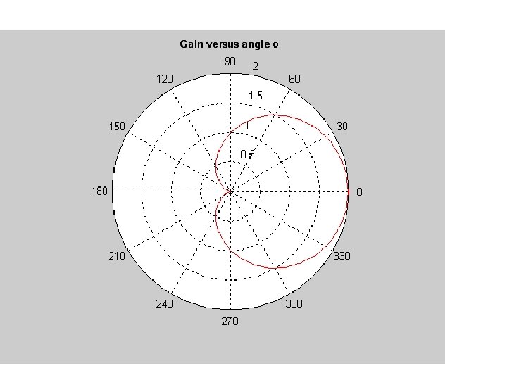
3. 5. 7 Polar Plots • polar(theta, r) • e. g. script file: microphone. m % Calculate gain versus angle g = 0. 5; theta = 0: pi/20: 2*pi; gain = 2*g*(1+cos(theta)); % Plot gain polar (theta, gain, 'r-'); title ('bf. Gain versus angle theta');

Plotting: Example 3. 6 plot_fileter. m Plot the amplitude and frequency response r = 16 k ∧∧∧ ∨ c = 1. 0 u. F C V 0 Vi A simple low-pass filter circuit

r = 16000; c = 1. 0 e-6; f = 1: 2: 1000; res = 1. / ( 1 + j*2*pi*f*r*c ); amp = abs(res); phase = angle(res); subplot(2, 1, 1); loglog(f, amp); title( 'Amplitude response' ); xlabel( 'Frequency (Hz)' ); ylabel( 'Output/Input ratio' ); grid on; subplot(2, 1, 2); semilogx(f, phase); title( 'Phase response' ); xlabel( 'Frequency (Hz)' ); ylabel( 'Output-Input phase (rad)'

3. 5. 8 Annotating and Saving Plots • Annotating – Editing tool – Text tool – Arrow tool – Line tool • Saving • Quiz 3. 3

Plotting Summary • plot(x, y) linear plot of vector y vs. vector x • title('text'), xlabel('text'), ylabel('text') labels the figure, x-axis and y-axis • grid on/off adds/removes grid lines • legend( 'string 1', 'string 2', 'string 3', . . . ) adds a legend using the specified strings • hold on/off allows/disallows adding subsequent graphs to the current graph

Plotting Summary • axis( [ xmin xmax ymin ymax ] ) sets axes’ limits • v = axis returns a row vector containing the scaling for the current plot • axis equal sets the same scale for both axes • axis square makes the current axis square in size

Plotting Summary • semilogy(x, y), semilogx(x, y), loglog(x, y) logarithmic plots of vector y vs. vector x • figure(k) makes k the current figure • subplot(m, n, p) breaks the figure window into an m-by-n matrix of small axes and selects the pth axes for the current plot • clf clears current figure

Two-Dimensional Plots • Additional Types of 2 D Plots: more than 20 types • Example: – line – Stem – Stair – Bar – Pie – compass

Two-Dimensional Plots: examples • Line plot x = -2: 0. 01: 4; y = 3. 5. ^(-0. 5*x). *cos(6*x); plot(x, y); line([0 0], [-3 3], 'color', 'r'); • Pie plot grades = [ 11 18 26 9 5 ]; pie(grades);

Two-Dimensional Plots: examples • Stairs plot y = 1988: 1994; s = [ 8 12 20 22 18 24 27 ]; stairs(y, s); • Stem plot y = 1988: 1994; s = [ 8 12 20 22 18 24 27 ]; stem(y, s);

Two-Dimensional Plots: examples • Vertical bar plot y = 1988: 1994; s = [ 8 12 20 22 18 24 27 ]; bar(y, s, 'r'); • Horizontal bar plot y = 1988: 1994; s = [ 8 12 20 22 18 24 27 ]; barh(y, s, 'g');

Two-Dimensional Plots: examples • Polar plot t = linspace(0, 2*pi, 200); r = 3 * cos(0. 5*t). ^2 + t; polar(t, r); • Compass plot u = [ 3 4 -2 -3 0. 5 ]; v = [ 3 1 3 -2 -3 ]; compass(u, v);

Two-Dimensional Plots: examples • Histogram x = randn(1, 100); hist(x, 10); hist(x, 20);

Two-Dimensional Plots: examples • Error bar plot x = 1: 10; y = sin(x); e = std(y) * ones(size(x)); errorbar(x, y, e);

Two-Dimensional Plots: Plotting Functions • Easy to plot: plot a function directly, without the necessity of creating intermediate data arrays. – ezplot(fun); – ezplot(fun, [xmin xmax], figure); • Example: ezplot('sin(x)/x', [-4*pi]); title('Plot of sinx/x'); grid on; • fplot

Three-Dimensional Plots: Line Plots • plot 3 • Example: – Test_plot. m t = 0: 0. 1: 10; x = exp(-0. 2*t). * cos(2*t); y = exp(-0. 2*t). * sin(2*t); plot(x, y, 'Line. Width', 2); title('bf. Two-Dimensional Line Plot'); xlabel('bfx'); ylabel('bfy'); axis square; grid on; – Test_plot 3. m t = 0: 0. 1: 10; x = exp(-0. 2*t). * cos(2*t); y = exp(-0. 2*t). * sin(2*t); plot 3(x, y, t, 'Line. Width', 2); title('bf. Three-Dimensional Line Plot'); xlabel('bfx'); ylabel('bfy'); zlabel('bftime'); grid on;

Three-Dimensional Plots: Surface, Mesh, Contour • Must create three equal-sized arrays • Data prepared – [x, y]=meshgrid(xstart: xinc: xend, ystart: yinc: yend); [x, y]=meshgrid(-4: 0. 2: 4, -4: 0. 2: 4); – Z=f(x, y) z = exp(-0. 5*(x. ^2+0. 5*(x-y). ^2)); • mesh(x, y, z), surf(x, y, z), contour(x, y, z) e. g. test_contour 2. m

3. 5 Three-Dimensional Plots: Line Plots • plot 3 • Example: – Test_plot. m t = 0: 0. 1: 10; x = exp(-0. 2*t). * cos(2*t); y = exp(-0. 2*t). * sin(2*t); plot(x, y, 'Line. Width', 2); title('bf. Two-Dimensional Line Plot'); xlabel('bfx'); ylabel('bfy'); axis square; grid on; – Test_plot 3. m t = 0: 0. 1: 10; x = exp(-0. 2*t). * cos(2*t); y = exp(-0. 2*t). * sin(2*t); plot 3(x, y, t, 'Line. Width', 2); title('bf. Three-Dimensional Line Plot'); xlabel('bfx'); ylabel('bfy'); zlabel('bftime'); grid on;

Three-Dimensional Plots: Surface, Mesh, Contour • Must create three equal-sized arrays • Data prepared – [x, y]=meshgrid(xstart: xinc: xend, ystart: yinc: yend); [x, y]=meshgrid(-4: 0. 2: 4, -4: 0. 2: 4); – Z=f(x, y) z = exp(-0. 5*(x. ^2+0. 5*(x-y). ^2)); • mesh(x, y, z), surf(x, y, z), contour(x, y, z) e. g. test_contour 2. m

2. 12 Examples • Script file: temp_conversion. m • Script file: calc_power. m • Script file: c 14_date. m

Example 2. 3 – temperature conversion • Design a MATLAB program that reads an input temperaturein degrees Fahrenheit, conberts it to an absolute temperature in kelvins, and writes out the result. Perform the following steps: 1. Prompt the user enter an input temperature in o. F; 2. Read the input temperature; 3. Calculate the temperature in kelvins from Equation 4. Write out the result, and stop

• temp_f=input('Enter the input temperature in degree Fahrenhert: ') • temp_k=(5/9)*(temp_f-32)+273. 15; • fprintf('%6. 2 f degree Fahrenhert=%6. 2 f kelvins. n', temp_f, temp_k);

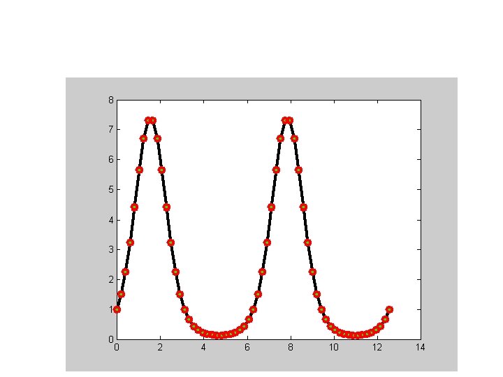
Examples 2. 4 Maximum Power Transfer to a Load Figure 2. 9 shows a voltage source V=120 V with an internal resistance Rs of 50Ω supplying a load of resistance RL, . Find the value of load resistance RL that will result in the maximum possible power being supplied by the Voltage source to the load. Haw much power will be supplied in this case? Also, plot the power supplied to the load as a function of the load resistance RL.

Examples 2. 4 Maximum Power Transfer to a Load In this program, we need to vary the load resistance RL and compute the power supplied to the load at each value of RL. The power supplied to the load resistance is given by the equation where I is the current supplied to the load. The current supplied to the load can be calculated by Ohm's law.

Examples 2. 4 Maximum Power Transfer to a Load The program must perform the following steps. 1. Create an array of possible values for the load resistance RL. The array will vary RL from 1Ω to 100Ω in 1Ω steps. 2. Calculate the current for each value of RL. 3. Calculate the power supplied to the load for each value of RL. 4. Plot the power supplied to the load for each value of RL, and determine the value of load resistance resulting in the maximum power.

Examples 2. 4 Maximum Power Transfer to a Load Now, we will demonstrate this program in MATLAB

Examples 2. 4 Maximum Power Transfer to a Load

2. 13 Debugging MATLAB Programs l Syntax errors v. Check spelling and punctuation l Run-time errors v. Check input data v. Can remove “; ” or add “disp” statements l Logical errors v. Use shorter statements v. Check typos v. Check units v. Ask your friends, instructor, parents, …

Review: Useful Commands v help command v lookfor keyword v which v clear v clc v diary filename v diary on/off v who, whos v Ctrl+c v… v% Online help Lists related commands Version and location info Clears the workspace Clears the command window Sends output to file Turns diary on/off Lists content of the workspace Aborts operation Continuation Comments

2. 14 Summary l Two data types: double and char l Assignment statements l Arithmetic calculations l Intrinsic functions l Input/output statements l Data files l Hierarchy of Operations

2. 14 Summary of Good Programming Practice v 1. Use meaningful variable names whenever possible. v 2. Create a data dictionary for each program. v 3. Use only lowercase letters in variable names. v 4. Use a semicolon at the end of all MATLAB assignment statements. v 5. Save data in ASCII format or MAT-file format. v 6. Save ASCII data files with a "dat" file extent and MAT-file with a “mat” extent. v 7. Use parentheses as necessary to make your equations clear and easy to understand. v 8. Always include the appropriate units with any values that you read or write in a program.

Homework • • Quiz 2. 1 (P. 30) Quiz 2. 2 (P. 38) Quiz 2. 3 (P. 44) Exercises – 1, 2, 3, 4, 5, 6, 7, 9, 11

plot:

• • th = [0: pi/50: 2*pi]'; a = [0. 5: 4. 5]; X = cos(th)*a; Y = sin(th)*sqrt(25 -a. ^2); plot(X, Y) axis('equal') xlabel('x'), ylabel('y') title('A set of Ellipses')