MATLAB LECTURE 4 Spatial Filtering IMAGE TYPES IN

MATLAB LECTURE 4 Spatial Filtering

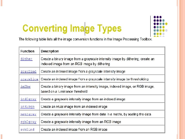
IMAGE TYPES IN THE TOOLBOX The Image Processing Toolbox supports four: Basic types of images: Indexed images Colored RGB images Intensity images Gray-scale Binary images Black and white

SUMMARY OF IMAGE TYPES AND NUMERIC CLASSES
; The type could")
SPATIAL FILTERING Filtering � Linear in Matlab filters: using fspecial(type, parameter); The type could be: Ø ‘average’ filter Ø ‘laplacian’ filter Ø ‘log’ filter � Non-linear filters: Ø Median filter: q medfilt 2

SPATIAL FILTERING We can create our filters by hand, or by using the fspecial function; this has many options which makes for easy creation of many deferent filters. fspecial(type, parameter) creates and returns common filters. filter 2(filter, image) apply the filter on the image
![AVERAGING FILTERING fspecial('average', [5, 7]) � will return an averaging filter of size 5](http://slidetodoc.com/presentation_image_h2/deed58242f22db3032c362b875b33399/image-7.jpg "AVERAGING FILTERING fspecial('average', [5, 7]) � will return an averaging filter of size 5")
AVERAGING FILTERING fspecial('average', [5, 7]) � will return an averaging filter of size 5 x 7 fspecial('average', 11) � will return an averaging filter of size 11 x 11 fspecial('average') � will return an averaging filter of size 3 x 3 (default)

AVERAGING FILTERING For example, suppose we apply the 3 x 3 averaging filter to an image as follows: >> c=imread('cameraman. tif'); >> f 1=fspecial('average'); >> cf 1=filter 2(f 1, c); We now have a matrix of data type double. To display this, we can do any of the following: � transform it to a matrix imshow(uint 8(cf 1)); of type uint 8, for use with imshow. � divide its values by 255 to obtain a matrix with values in the 0. 1 -1. 0 range, for use with imshow(cf 1/255); � use mat 2 gray to scale the imshow(mat 2 gray(cf 1)); result for display. >> figure, imshow(c), figure, imshow(cf 1/255)
 and 6. 4(b).")
AVERAGING FILTERING will produce the images shown in figures 6. 4(a) and 6. 4(b). The averaging filter blurs the image; the edges in particular are less distinct than in the original. The image can be further blurred by using an averaging filter of larger size. This is shown in the following figures:

AVERAGING FILTERING

AVERAGING FILTERING

FREQUENCIES; LOW AND HIGH PASSFILTERS High pass filter if it passes over the high frequency components, and reduces or eliminates low frequency components. Low pass filter if it passes over the low frequency components, and reduces or eliminates high frequency components. Both are mainly used for noise reduction, sharpen, or smooth the image. May be used for edge detection. The output may be the same for the tow types. sharp smooth (low), smooth sharp (high)
; >> cf=filter 2(f, c); >> imshow(cf/255); >>")
FREQUENCIES; LOW AND HIGH PASSFILTERS >> f=fspecial('laplacian'); >> cf=filter 2(f, c); >> imshow(cf/255); >> f 1=fspecial('log'); >> cf 1=filter 2(f 1, c); >> figure, imshow(cf 1/255);
 is")
HIGH PASS FILTERING The images are shown in figure 6. 5. Image (a) is the result of the Laplacian filter; image (b) shows the result of the Laplacian of Gaussian (log) filter.

MEDIAN FILTER medfilt 2 Median filtering is a nonlinear operation often used in image processing to reduce "salt and pepper" noise. What is "salt and pepper" noise ? � it is randomly occurring of white and black pixels. n = imnoise(i, 'salt & pepper‘, 0. 2); imshow(n); The default is 0. 05 Higher value more noise
 performs median filtering of the matrix A using")
MEDIAN FILTER B = medfilt 2(A) performs median filtering of the matrix A using the default 3 -by-3. Examples � Add salt and pepper noise to an image and then restore the image using medfilt 2. >>I = imread('eight. tif'); >>J = imnoise(I, 'salt & pepper', 0. 2); >>K = medfilt 2(J); >>imshow(J), figure, imshow(K)
- Slides: 16