MATLAB Environment Chapter 2 contd MATLAB for Engineers

MATLAB Environment Chapter 2 (contd. ) MATLAB for Engineers 3 E, by Holly Moore. © 2011 Pearson Education, Inc. , Upper Saddle River, NJ. All rights reserved. This material is protected by Copyright and written permission should be obtained from the publisher prior to any prohibited reproduction, storage in a retrieval system, or transmission in any form or by any means, electronic, mechanical, photocopying, recording, or likewise. For information regarding permission(s), write to: Rights and Permissions Department, Pearson Education, Inc. , Upper Saddle River, NJ 07458.

Array Operations • Using MATLAB as a glorified calculator is OK, but its real strength is in matrix manipulations

To create a row vector, enclose a list of values in brackets

You may use either a space or a comma as a “delimiter” in a row vector

Use a semicolon as a delimiter to create a new row

Hint: It’s easier to keep track of how many values you’ve entered into a matrix, if you enter each row on a separate line. The semicolons are optional

Shortcuts • While a complicated matrix might have to be entered by hand, evenly spaced matrices can be entered much more readily. The command b= 1: 5 or the command b = [1: 5] both return a row matrix

The default increment is 1, but if you want to use a different increment put it between the first and final values

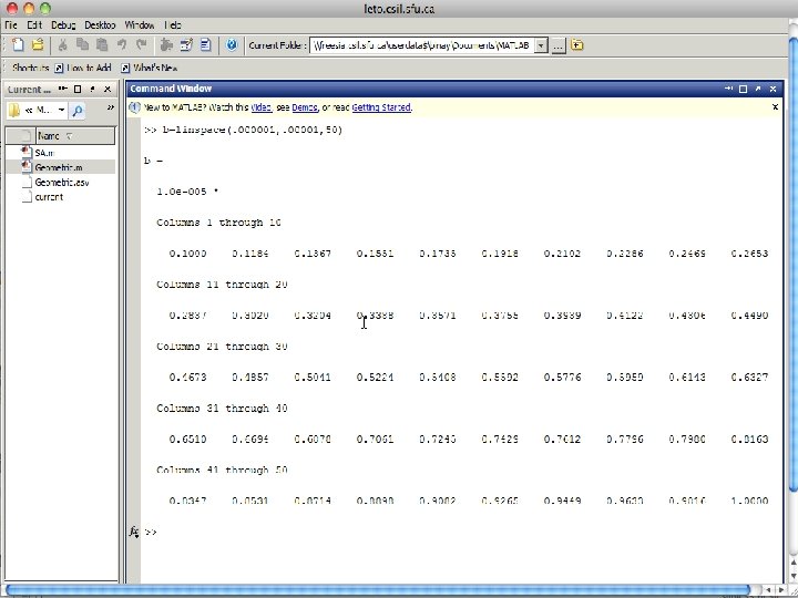
To calculate spacing between elements use… • linspace • logspace

number of elements in the array Initial value in the array Final value in the array

number of elements in the array Initial value in the array expressed as a power of 10 Final value in the array expressed as a power of 10

It is a common mistake to enter the initial and final values into the logspace command, instead of entering the corresponding power of 10

Hint • You can include mathematical operations inside a matrix definition statement. • For example a = [0: pi/10: pi]

Mixed calculations between scalars and arrays • Matrices can be used in many calculations with scalars • There is no confusion when we perform addition and subtraction • Multiplication and division are a little different • In matrix mathematics the multiplication operator (*) has a very specific meaning

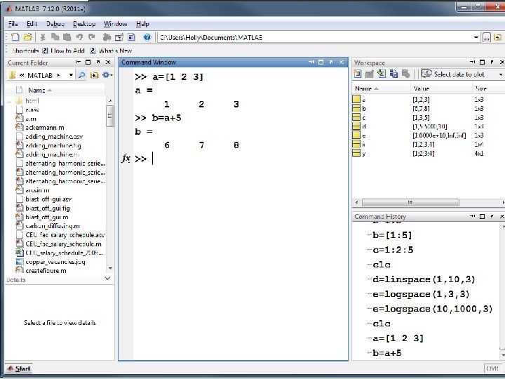
Addition between arrays is performed on corresponding elements

Multiplication between arrays is performed on corresponding elements if the. * operator is used

MATLAB interprets * to mean matrix multiplication. The arrays a and b are not the correct size for matrix multiplication in this example

Array Operations • Array multiplication • Array division • Array exponentiation In each case the size of the arrays must match . *. /. ^

The matrix capability of MATLAB makes it easy to do repetitive calculations • For example, assume you have a list of angles in degrees that you would like to convert to radians. – First put the values into a matrix. – Perform the calculation

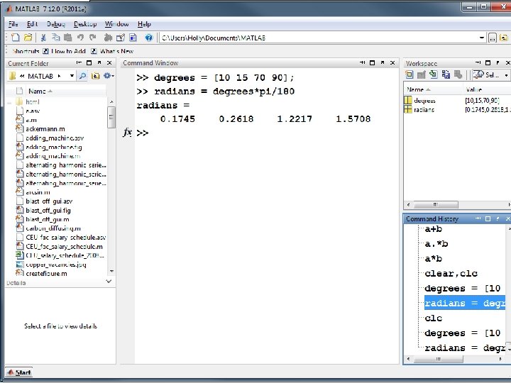
Either the * or the. * operator can be used for this problem, because it is composed of scalars and a single matrix The value of pi is built into MATLAB as a floating point number, called pi

More about pi • Because pi is an irrational number, it can not be expressed exactly with a floating point representation • The MATLAB constant, pi, is really an approximation. • If you find sin(pi) MATLAB returns a very small number.

Transpose • The transpose operator changes rows to columns or vice versa.

The transpose operator makes it easy to create tables

table =[degrees; radians]’ would have given the same result

The transpose operator works on both one dimensional and two dimensional arrays

Number Display • Scientific Notation – Although you can enter any number in decimal notation, it isn’t always the best way to represent very large or very small numbers – In MATLAB, values in scientific notation are designated with an e between the decimal number and exponent. (Your calculator probably uses similar notation. )

It is important to omit blanks between the decimal number and the exponent. For example, MATLAB will interpret 6. 022 e 23 as two values (6. 022 and 1023 )

Display Format • Multiple display formats are available • No matter what display format you choose, MATLAB uses double precision floating point numbers in its calculations • MATLAB handles both integers and decimal numbers as floating point numbers

Default • The default format is called short • If an integer is entered it is displayed without trailing zeros • If a floating point number is entered four decimal digits are displayed

Other formats • Changing the format affects all subsequent displays – format long results in 14 decimal digits – format bank results in 2 decimal digits – format short returns the display to the default 4 decimal digits

Really Big and Really Small • When numbers become too large or too small for MATLAB to display using the default format, it automatically expresses them in scientific notation • You can force scientific notation with – format short e – format long e

Common Scale Factor • For long and short formats, a common scale factor is applied to the entire matrix if some of the elements become very large, or very small. This scale factor is printed along with the scaled values.

Common Scale Factor

Section 2. 4 Saving Your Work • If you save a MATLAB session performed in the command window, all that is saved are the values of the variables you have named

Variables are saved, not the commands in the command window

Save either by using the file menu or. . . Save with a command in the command window

MATLAB automatically saves to a. mat file • If you want to save to another format, such as. dat, you need to explicitly tell the program save <file_name> <variable_list> -ascii Again – Remember that the only things being saved are the values stored in the workspace window – not the commands from the command window

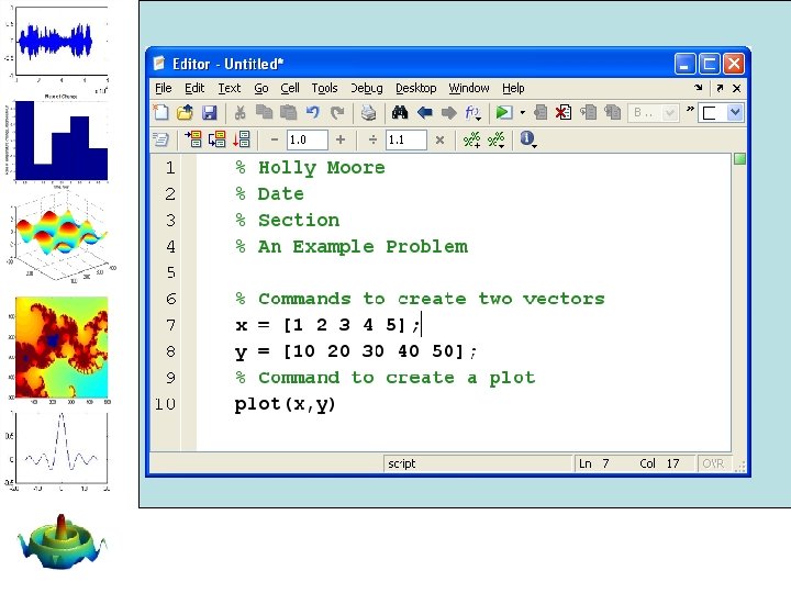
Script M-files • If you want to save your work, (the commands you entered) you need to create an M-file • File->New->M-file • Type your commands in the edit window that opens

• The file can be saved into the current folder/directory • It runs in the command window

Save the file using the save icon, or the file menu

You can dock the editing window with the MATLAB desktop, by using the docking arrow

This arrangement is often easier to use

I saved this file as example. m Notice that it now appears in the current directory When I execute the file, the figure appears on top of the MATLAB desktop

The figure window can also be docked onto the MATLAB desktop, using the docking arrow

Notice that the command history window is hidden underneath the figure, but can be accessed with the tab

Comments • Be sure to comment your code – Add your name – Date – Section # – Assignment # – Descriptions of what you are doing and why

The % sign identifies comments You need one on each line

Summary • • Introduced the MATLAB Windows Basic matrix definition Save and retrieve MATLAB data Create and use script M-files