MATLAB Basics MATLAB Workspace environment address space where

MATLAB Basics
 where all variables reside } Most recent answer")
MATLAB } Workspace: environment (address space) where all variables reside } Most recent answer is always stored in variable ans } “%” marks the beginning of a comment line } Three windows } Command window: used to enter commands and data } Edit window: used to create and edit M-files (programs) such as the factor. For example, we can use the editor to create factor. m } Graphics window(s): used to display plots and graphics 2

Command Window } Used to enter commands and data, prompt “>>” } Allow the use of MATLAB as a calculator when commands are typed in line by line, e. g. , >> a = 77 -16 ans = 61 >> b = a * 10 ans =610 3

System Commands } who/whos: list all variables in the workspace } clear: remove all variables from the workspace } clc: clear all input and output (history) from the Command Window display } computer: list the system MATLAB is running on } version: list the toolboxes (utilities) available 4

Variable Names } A valid variable name starts with a letter, followed by letters, digits, or underscores } Case sensitive, up to 31 alphanumeric characters (letters, numbers) and the underscore (_) symbol } Reserved words } } } } } ans eps realmax realmin pi i j inf nan Most recent answer Floating point relative accuracy Largest positive floating point number Smallest positive floating point number 3. 1415926535897. . Imaginary unit Infinity Not-a-Number 5
 } } isnan isinf isfinite why True for")
Variable Names } Reserved words (cont’d) } } isnan isinf isfinite why True for Not-a-Number True for infinite elements True for finite elements Succinct answer 6

Data Display } The format command allows you to display real numbers } short - scaled fixed-point format with 5 digits } long - scaled fixed-point format with 15 digits for double and 7 digits for single } short eng - engineering format with at least 5 digits and a power that is a multiple of 3 (useful for SI prefixes) } The format does not affect the way data is stored internally 7

Data Display: Examples } >> format short; pi ans = 3. 1416 >> format long; pi ans = 3. 14159265358979 >> format short eng; pi ans = 3. 1416 e+000 >> pi*10000 ans = 31. 4159 e+003 } Note: the format remains the same unless another format command is issued 8

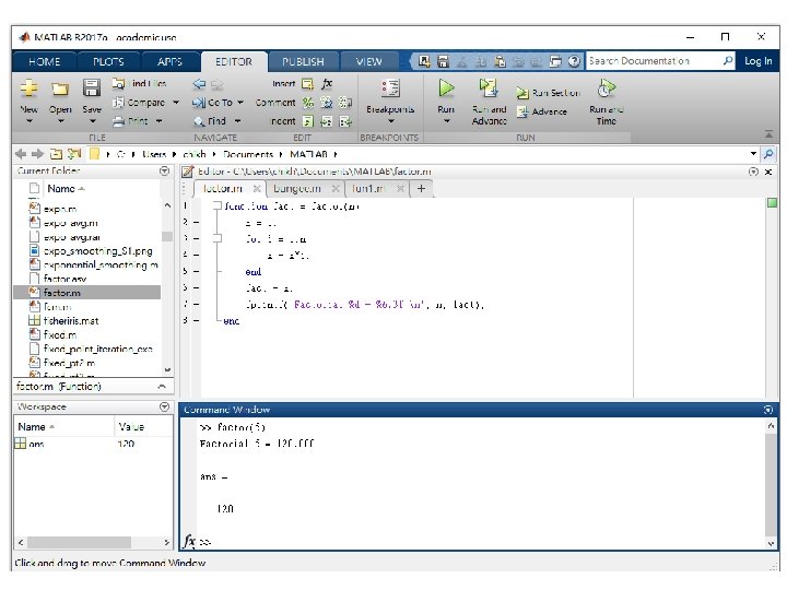
Script File: Set of MATLAB Commands } Example: the script factor. m http: //bit. ly/2 VYEXmd function fact = factor(n) x = 1; for i = 1: n x = x*i; end fact = x; %fprintf('Factorial %d = %6. 3 f n', n, fact); end } How the script works? } Type its name (without the. m) in the command window; } Select the Debug, Run (or Save and Run) command in the editing window; or } Hit the F 5 key while in the editing window 9

File-Naming Rule http: //bit. ly/3 a. VT 53 Z 11

Array } Vector = one-dimensional array, matrix = twodimensional array >> a = [1 2 3 4 5] % specify elements of the array individually separated by spaces or commas a= 1 2 3 4 5 >> a = 1: 2: 10 % specify, the first element, the increment, and the largest possible element a= 1 3 5 7 9 >> a = [1 3 5 7 9] % specify elements separated by commas or spaces a= 1 3 5 7 9 12

Array } Arrays are stored column wise (column 1, followed by column 2, etc. ) } A semicolon marks the end of a row >> a = [1; 2; 5] a= 1 2 5 13
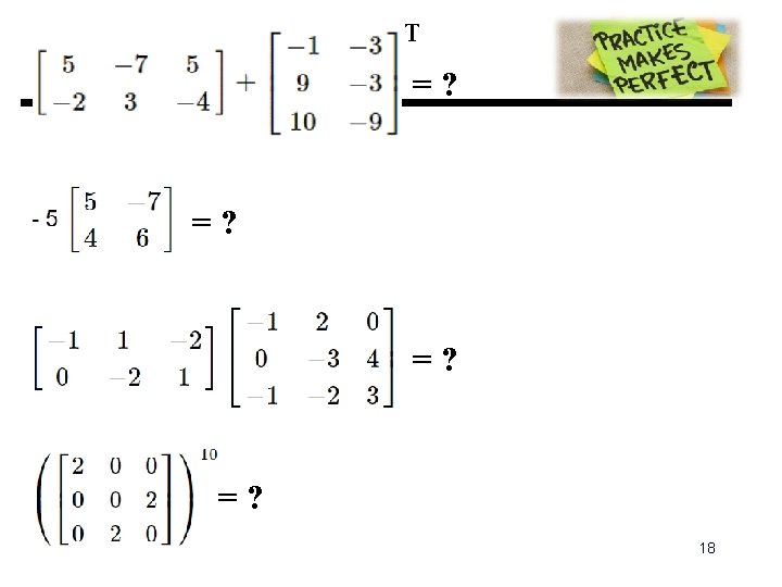
 operator transform rows in columns and columns")
Transpose of an Array } Transpose (') operator transform rows in columns and columns in rows >> b = [2 9 3; 4 16 5; 6 13 7; 8 19 9; 10 11 11] b= 2 9 3 4 16 5 6 13 7 8 19 9 10 11 11 >> b' % Transpose of matrix b ans = 2 4 6 8 10 9 16 13 19 11 3 5 7 9 11 14
 operator transform rows in columns and columns")
Transpose of an Array } Transpose (‘) operator transform rows in columns and columns in rows; >> c = [2 9 3 4 16; 5 6 13 7 8; 19 9 10 11 11] c= 2 9 3 4 16 5 6 13 7 8 19 9 10 11 1 15
 } Both arrays must have the same number of elements")
Element-by-Element Array Operations (1/2) } Both arrays must have the same number of elements } multiplication. * } division. / } exponentiation ^ (notice the “. ” before “*”, “/”, or “^”) >> b. * b ans = 4 81 9 16 25 36 169 49 64 361 81 100 121 16
 } Both arrays must have the same number of elements")
Element-by-Element Array Operations (2/2) } Both arrays must have the same number of elements >> b. / b ans = 1 1 1 1 http: //bit. ly/2 Q 1 ib. X 5 17
")
Identify an Element of an Array } Assignment of array elements >> b(4, 2) % element in row 4 column 2 of matrix b ans = 19 >> b(9) % the 9 -th element of b (recall that elements are stored column wise) ans = 19 >> b(5) % the 5 -th element of b (recall that elements are stored column wise) ans = 10 >> b(17) ? ? ? Attempted to access b(17); index out of bounds because numel(b)=15. >> whos Name Size Bytes Class Attributes 19 b 5 x 3 120 double
: create an r")
Array Creation – with Built-in Functions } } } zeros(r, c): create an r row by c column matrix of zeros(n): create an n by n matrix of zeros ones(r, c): create an r row by c column matrix of ones(n): create an n by n matrix ones help elmat: give a list of the elementary matrices 20
 } Create a linearly spaced array of points start: diffval: limit")
Colon Operator (1/2) } Create a linearly spaced array of points start: diffval: limit } start first value in the array } diffval difference between successive values in the array } limit boundary for the last value } Example >> 1: 0. 6: 3 ans = 1. 0000 1. 6000 2. 2000 2. 8000 } If diffval is omitted, the default value is 1 >> 3: 6 ans = 3 4 5 6 21
 } To create a decreasing series, diffval is negative >> 5:")
Colon Operator (2/2) } To create a decreasing series, diffval is negative >> 5: -1. 2: 2 ans = 5. 0000 3. 8000 2. 6000 } If start+diffval > limit for an increasing series or start+diffval < limit for a decreasing series, an empty matrix is returned >> 5: 2 ans = Empty matrix: 1 -by-0 } To create a column, transpose the output of the colon operator, not the limit value; that is, (3: 6)’ not 3: 6’ 22
: create a linearly spaced row")
Array Creation: linspace } linspace(x 1, x 2, n): create a linearly spaced row vector of n points between x 1 and x 2 >> linspace(0, 1, 6) ans = 0 0. 2000 0. 4000 0. 6000 0. 8000 1. 0000 } If n is omitted, 100 points are created } To generate a column, transpose the output of the linspace command 23
: create a logarithmically spaced row")
Array Creation: logspace } logspace(x 1, x 2, n): create a logarithmically spaced row vector of n points between 10 x 1 and 10 x 2 >> logspace(-1, 2, 4) ans = 0. 1000 1. 0000 100. 0000 } If n is omitted, 100 points are created } To generate a column vector, transpose the output of the logspace command 24

Arithmetic Operations on Scalars and Arrays } Operators in order of priority ^ 4^2 = 16 - -8 = -8 * 2*pi = 6. 2832 / pi/4 = 0. 7854 62 = 0. 3333 + 3+5 = 8 - 3 -5 = -2 25

Complex Numbers } Arithmetic operations can be performed on complex numbers x = 2+i*4; (or 2+4 i, or 2+j*4, or 2+4 j) y = 16; 3*x ans = 6. 0000 +12. 0000 i x+y ans = 18. 0000 + 4. 0000 i x' ans = 2. 0000 - 4. 0000 i 26

Quadratic Equations } Example: Solve the equation ax 2+bx+c=0 } Roots } Special case: a=0 and b=0 bx + c=0 x = - c/b } Special case: b=0 ax 2+ c=0 27
 % Input: coefficients (a, b,")
Program for Solving Quadratic Equations function quadroots(a, b, c) % Input: coefficients (a, b, c) of a quadratic equation % Output: real and imaginary parts of the solution (R 1, I 1), (R 2, I 2) if a==0 % special case if b ~= 0 x 1 = -c/b else error('a and b are zero') end else d = b^2 - 4*a*c; if d > = 0 % real roots R 1 = (-b + sqrt(d))/(2*a) R 2 = (-b - sqrt(d))/(2*a) else % complex roots R 1 = -b/(2*a) I 1= sqrt(abs(d))/(2*a) R 2 = R 1 I 2= -I 1 end

Important Subjects https: //www. tutorialspoint. com/matlab/ 29

Important Subjects 30

} A perfect number n is a positive integer in which sum of all positive divisors excluding n is equal to n. For instance, 6=1+2+3, so 6 is a perfect number, whereas 8 is not (8≠ 1+2+4. ) Write a MATLAB program that finds all the perfect numbers smaller than a given integer. An example screenshot of the program is shown below. 31

Practice: Read/Visualize Data from A. xls File %Program: spending. Plots. m %Note: Distribution of data points can be viewed as the % relationship of x to y on the plane clear all; [~, month] = xlsread('expenditures. xlsx', 'Year 2019', 'A 2: A 13'); x = 0: 1: 11; [y] = xlsread('expenditures. xlsx', 'Year 2019', 'B 2: B 13'); plot(x, y); %plot(x, y, 'o'); title('Monthly Expenditure of Year 2019'); %set(gca, 'XTick', [0: 11], 'xticklabel', month) %xlim([0 11]) %xlabel 'Month'; %ylabel 'Spending'; %print(gcf, '-dpng', 'spending. Plots. png', '-r 0'); http: //bit. ly/2 TQ 64 Ny
 times and")
} Write a MATLAB program that simulates throwing a die n (=120) times and shows outcomes } The program counts and displays how many times each face of pips (1. . 6) has appeared throughout the simulation } Animation-like presentation is useful to demonstrate changes of outcome over time } Think about possible types of plots illustrating results } You are advised to observe whether random numbers were generated evenly } Examine also whether your program gets the same sequence of random numbers when invoked at different times } Extend your program to allow for 2 or 3 dice 33

} Revise the previous code so as to show the outcome of each trial

} Revise the previous code so as to show the relative frequency of each face of pips versus n } Relative frequency n: # of experiments under identical condition k: counter index N 1: # of 1 -pip faces N 2: # of 2 -pip faces …in n trials … N 6: # of 6 -pip faces …probability of the outcome k


Practice: Ordinary Differential Equation } Recall: Bungee jumper example http: //bit. ly/2 TGMAMD 37 http: //www. eng. auburn. edu/~tplacek/courses/3600/ode 45 waterloo. pdf

Read Textbook Chapters 2 and 3 38
- Slides: 38