MATLAB Basic Course for EEG analysis 20 02

MATLAB Basic Course for EEG analysis 20. 02. 01 뇌파연구회 Kwang Su Cha, Ki-Young Jung Department of Neurology , Seoul National University Hospital, South Korea
 1. EEGLAB Download http: //sccn. ucsd. edu/eeglab/currentversion/eeglab_current. zip 2")
1 Initial set-up (EEGLAB toolbox) 1. EEGLAB Download http: //sccn. ucsd. edu/eeglab/currentversion/eeglab_current. zip 2 2. Click “Set path” 3. Add with subforlders 4. Select EEGLAB folder 실습 자료 Download path: … 3 4

MATLAB • MATLAB is an abbreviation for “MAtrix LABoratory" • Data analysis • Algorithm development • Modeling • Statistics • Graphic expression • …

How to analyze an EEG Analysis Data • Software BESA, Curry… • → Intuitive/integrative, but high computational load Matlab Coding (Field trip) GUI (EEGLAB, Brainstorm…) • Python MNE → Easy, but expensive/restrictive → Faster (useful to big data/high computation), but uncomfortable Results

Why we use MATLAB for EEG analysis Data Integrative analysis using MATLAB Analysis results Statistics Figures Data reconstruction

What we will learn in this course EEG Recording EEG raw data Data loading, Initialization EEG data (preprocessed) Interpolation, Artifact rejection … Results Analysis (PSD, FC …) Figures Expression (Histogram, Error-bar, Time-course, Draw waveform)

Introduction to MATLAB

Window constitution
 “Error: expected single or double Solution! >> double(변수)")
MATLAB basic Class (참고만!) “Error: expected single or double Solution! >> double(변수)

Write matrix • A matrix can be created in MATLAB as follows (note the “commas(or blanks)” AND “semicolons”): » matrix = [1 , 2 , 3 ; 4 , 5 , 6 ; 7 , 8 , 9] matrix = 1 4 7 2 5 8 3 6 9

Matrix indexing

Matrix indexing
 또는 (channels,")
Construct matrix for EEG data • EEG Data 구조 (channels, raw data) 또는 (channels, raw data/epoch, epochs) • Matrix expression channels hs oc p e 또는 channels Sampling rate: 400 Hz raw data Data length: 60 s Data length: 24, 000 point raw data

Matrix appending matrix A = 1 4 7 2 5 8 matrix B = 3 6 9 10 13 16 11 14 17 12 15 18 • Append matrix C = [A, B] 1 4 7 2 5 8 3 6 9 10 13 16 matrix C = [A; B] 11 14 17 12 15 18 10 13 16 11 14 17 12 15 18
 Sub A의 matrix size: (300 pt, 50 trials)")
Matrix appending: example • Q 1) Sub A의 matrix size: (300 pt, 50 trials) 이고 Sub B의 matrix size: (300 pt, 35 trials) 일때 Sub A +Sub B 병합한 Sub C(300 pt, 85 trials)를 생성? >> Sub C = [Sub A; Sub B]; • Q 2) Sub A의 matrix size: (300 pt, 19 ch, 50 trials) & Sub B의 matrix size: (300 pt, 19 ch, 35 trials) Sub A +Sub B 병합한 Sub C(300 pt, 19 ch, 85 trials)를 생성? >> Sub C = cat(3, Sub A, Sub B);
 Subject 2 (c, t, n, 2) (n ) Subject")
Matrix array (ex. ERP data) Subject 2 (c, t, n, 2) (n ) Subject 1 (c, t, n, 1) u. V u. V tri al s u. V u. V u. V u. V u. V time-point (t) u. V u. V u. V u. V u. V u. V channels (c) u. V u. V . . .
 u. V")
Different number of trials across subjects Subject 2 (c, t, m, 2) u. V u. V u. V u. V u. V 0 0 0 u. V u. V u. V u. V u. V u. V 0 0 u. V time-point (t) 0 u. V channels (c) u. V (m u. V s u. V al u. V tri al s u. V tri (n ) ) Subject 1 (c, t, n, 1) u. V 0 u. V 0 . . .
 {1} {2} {3}")
Cell & Structure array • Cell array • Structure array (참고!) {1} {2} {3} Access: patient{1}(data) patient{2}(data) Patient{3}(data) Access: patient. name(data) patient. billing(data) patient. test(data)
 Data save (incorrect) Data save (correct) Sub 1: sub_total(: , :")
Cell array (중요!) Data save (incorrect) Data save (correct) Sub 1: sub_total(: , : , 1) = sub 1(19, 600, 35); Sub 1: sub_total{1} = sub 1(19, 600, 35); Sub 2: sub_total(: , : , 2) = sub 2 (19, 600, 25); Sub 2: sub_total{2} = sub 2 (19, 600, 25); Sub 3: sub_total(: , : , 3) = sub 3 (19, 600, 10); Sub 3: sub_total{3} = sub 3 (19, 600, 10); Sub 4: sub_total(: , : , 4) = sub 4 (19, 600, 30); Sub 4: sub_total{4} = sub 4 (19, 600, 30); Sub 5: sub_total(: , : , 5) = sub 5 (19, 600, 5); Sub 5: sub_total{5} = sub 5 (19, 600, 5); Sub 6: sub_total(: , : , 6) = sub 6 (19, 600, 15); Sub 6: sub_total{6} = sub 6 (19, 600, 15); … … ___________________ sub_total 의 size: (19, 600, 35, 6) sub_total의 size: {6}(19, 600, nsub)

Matrix operation
")
Matrix operation (matrix x matrix)
 반드시!")
Matrix operation (matrix by matrix) 반드시!

Operators == ~= < <= > >= equal not equal less than or equal greater than or equal & | ~ AND OR NOT pi j i 3. 14159265… imaginary unit, same as j
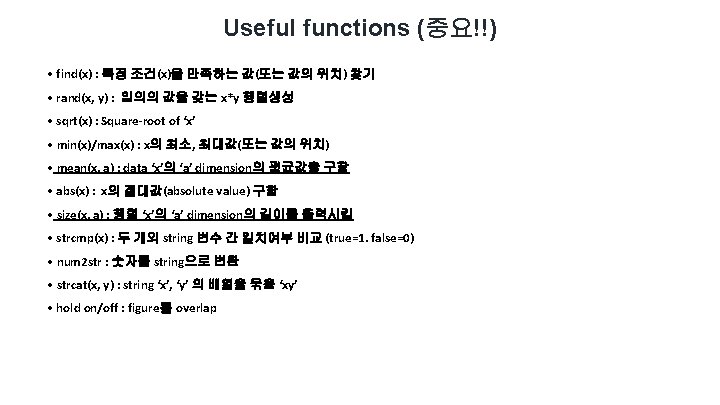
 • mean(x, a) : data ‘x’의 ‘a’ dimension의 평균값을 구함 matrix")
Useful functions (중요!!) • mean(x, a) : data ‘x’의 ‘a’ dimension의 평균값을 구함 matrix A matrix B >> matrix A= (channels, raw data) >> matrix B= mean(A, 1) • size(x, a) : 행렬 ‘x’의 ‘a’ dimension의 길이를 출력시킴 >> matrix A= (channels, raw data) >> B= size(A, 2) matrix A

HELP is the best Teacher of your MATLAB study !!!!!!!

Syntax – for, if for loop for variable = expression statements end if, elseif if expression 1 statements 1 elseif expression 2 statements 2 else statements 3 end

Syntax – for, if for loop for i = 1: 10 j= j + 1; end if, elseif a = [1, 2]; if a==1 b=min(a); elseif (a==2)&(a==1) b=max(a); elseif (a==2)|(a==1) b=mean(a); else b=a; end >> b?
; for k =")
Examples – If, for loop if, elseif x = rand(4, 1); for k = 1: 1: 4 avg_x = mean(x); y(1, k) = 2 * x(k, 1); end if avg_x >. 3 y =. 5 * x ; elseif avg_x <. 3 y = 2 * x; else equal to…. y = x; y = 2 * x’ ; end
![About “Function” Syntax function [out 1, out 2, . . . ] = funname(in](http://slidetodoc.com/presentation_image_h2/764f35c46ad2aa16194f40e9b151559d/image-32.jpg "About “Function” Syntax function [out 1, out 2, . . . ] = funname(in")
About “Function” Syntax function [out 1, out 2, . . . ] = funname(in 1, in 2, . . . ) Output variables Input variables Function name Ex) Convolution function [y] = conv_m(x, nx, h, nh) nyb = nx(1)+nh(1); nye = nx(length(x)) + nh(length(h)); ny = [nyb: nye]; y = conv(x, h);

Application to EEG data
 방법 1 (숫자): >>textread(‘filename. txt’) 방법 2 (숫자 &")
Load raw data (. txt) 방법 1 (숫자): >>textread(‘filename. txt’) 방법 2 (숫자 & 문자열): >>Fp=fopen(‘filename. txt’, ‘r’); >>VS_1=textscan(Fp, '%f‘, ‘Header. Lines’, 5); >>Fclose(Fp);
![Load data (. edf, . set) EDF file loading: >> EEG = pop_biosig([경로, 이름]);](http://slidetodoc.com/presentation_image_h2/764f35c46ad2aa16194f40e9b151559d/image-35.jpg "Load data (. edf, . set) EDF file loading: >> EEG = pop_biosig([경로, 이름]);")
Load data (. edf, . set) EDF file loading: >> EEG = pop_biosig([경로, 이름]); SET file loading: >> EEG = pop_loadset(경로, 이름); 이 때, EEG는 struct 형태 Data 불러오기 >> Data = EEG. data event 불러오기 >> events = EEG. event
![Load data (. xls, . cvs) [numbers, strings]=xlsread(‘경로. csv');](http://slidetodoc.com/presentation_image_h2/764f35c46ad2aa16194f40e9b151559d/image-36.jpg "Load data (. xls, . cvs) [numbers, strings]=xlsread(‘경로. csv');")
Load data (. xls, . cvs) [numbers, strings]=xlsread(‘경로. csv');
![Load data (. xls, . cvs) [numbers, strings]=xlsread(‘경로. csv'); numbers strings](http://slidetodoc.com/presentation_image_h2/764f35c46ad2aa16194f40e9b151559d/image-37.jpg "Load data (. xls, . cvs) [numbers, strings]=xlsread(‘경로. csv'); numbers strings")
Load data (. xls, . cvs) [numbers, strings]=xlsread(‘경로. csv'); numbers strings
인 행렬; >> results")
Data handling - reshape: reshape array Data = size가 (19, 18000)인 행렬; >> results = reshape(Data, [19, 600, 30]); 결과: results는 (19, 600, 30)로 재구성; - squeeze: remove singleton dimensions >> results = mean(Data(19, 600, 30), 1); 결과 1: results는 (1, 600, 30)로 구성; >> results 2 = squeeze(results); 결과 2: results는 (19, 30)로 구성; - repmat: replicate and tile array Data = size가 (19 , 1)인 행렬; >> results = repmat(Data, [1, 300]); 결과: results는 (19, 300)의 크기로 복제;

Load EDF files: example 폴더구성은 아래 그림과 같고, 각 edf 파일 내 raw data 구성은 (19 ch, 1800 pt) 임 모든 피험자 데이터에 대해 1 개의 Matrix array로 정리 Group_data={10 sub}(19 ch, 600 pt, 3 epochs); - control_num=[1, 4, 5, 6, 7, 8, 9, 11, 12, 15]; - control_name={‘lys’, ‘yse’, ‘kih’, ‘cws’, ‘adh’, ‘jwe’, phi’, ‘lyj’, ‘pyj’, ‘ljc’}; - for sub=1: 10 filepath=['C: test_data’]; filename=[strcat('sub_', num 2 str(control_num(sub)), ‘_’, control_name{sub}, ’. edf’)]; EEG = pop_biosig([filepath, filename]); Data=EEG. data; group_data{sub}(: , : )=reshape(Data, [19, 600. 3]); clear Data, EEG filepath filename - end
인 행렬을")
Matrix export to. edf or. set - Data 구성이 (19 ch, 18000 pt)인 행렬을 edf 또는 set 형태로 저장 - 필요한 정보: sampling rate, channel information - (19, 600)형태의 1로 구성된 임의의 행렬 생성 >> Data=ones(19, 600); - EEGLAB format으로 변환 >> EEG = pop_importdata('dataformat', 'matlab', 'nbchan', 19, 'data', Data, 'srate', 200, 'pnts', 0, 'xmin', 0, 'chanlocs', 'snuh_19 ch. ced'); - 1) EDF로 저장 >> pop_writeeeg(EEG, 'C: matlab. edf', 'TYPE', 'EDF'); - 2) SET으로 저장 >> EEG = pop_saveset( EEG, 'filename', 'matlab. set', 'filepath', 'C: ');
 • hold on, off • 2 D")
Plot figures • figure • plot(x, y) • hold on, off • 2 D (time-frequency map) imagesc(data)

Plot figures: example 연도별 체중변화 yr 2009 2010 2011 2012 2013 2014 2015 2016 2017 2018 2019 sub 1 70 68 69 72 75 76 74 68 65 66 64 sub 2 80 78 77 75 73 71 68 79 85 87 89 >> yr = [2009, 2010, 2011, 2012, 2013, 2014, 2015, 2016, 2017, 2018, 2019] >> sub_1 = [70, 68, 69, 72, 75, 76, 74, 68, 65, 66, 64] >> sub_2 = [80, 78, 77, 75, 73, 71, 68, 79, 85, 87, 89]
 >> hold on >> plot(yr, sub_2) 숙지할 필요 X History 이용!!")
>> plot(yr, sub_1) >> hold on >> plot(yr, sub_2) 숙지할 필요 X History 이용!! >> Parent 1=figure >> axes 1 = axes('Parent', Parent 1, 'Font. Size', 16, 'Font. Name', 'Arial'); >> xlim(axes 1, [2008 2020]); >> ylim(axes 1, [50 100]); >> hold(axes 1, 'on'); >> ylabel('kg'); >> xlabel('year'); >> plot 1 = plot(yr, [sub_1; sub_2], 'Marker. Size', 10, 'Line. Width', 2); >> set(plot 1(1), 'Display. Name', 'sub 1', 'Marker', 'o', 'Color', [0 0 1]); >> set(plot 1(2), 'Display. Name', 'sub 2', 'Marker', 'x', 'Line. Style', '--', . . . 'Color', [1 0 0]);

Useful toolbox for plotting • circstat • barwitherr • shaded. Error. Bar • not. Box. Plot

Useful toolbox for plotting
![Other useful functions - Paired-sample t-test >> [h, p, ci, stats] = ttest(x, y);](http://slidetodoc.com/presentation_image_h2/764f35c46ad2aa16194f40e9b151559d/image-46.jpg "Other useful functions - Paired-sample t-test >> [h, p, ci, stats] = ttest(x, y);")
Other useful functions - Paired-sample t-test >> [h, p, ci, stats] = ttest(x, y); - Independent t-test >> [h, p, ci, stats] = ttest 2(x, y); - Non-parametric (Wilcoxon/Mann-Whitney) >> [p, h, stats] = ranksum(x, y) - Linear regression >> [r, m, b] = regress(x, y) - Correlation >> [rho, pval] = corr(x, y) % Pearson, Kendall, Spearman

Deep Learning Toolbox - MATLAB

Practice

Dataset: resting-state EEG • Subjects: 1 healthy control • Sampling rate: 400 Hz • Data length: 60 s • 60 channel EEG with linked-mastoid references (10 -10 systems)
 (Channels X length) Step")
Practice: resting-EEG - Step 1: load EEG dataset (function: load) (Channels X length) Step 2: segmentation (function: reshape) (Channels X epoch length X epochs) Step 3: DC offset removal (function: repmat) (Channels X epoch length X epochs) – DC offset - Step 4: ensemble average (function: mean) (Channels X epoch length) - Step 5: draw EEG time-series (function: plot) -

Initial set-up

Step 1: load EEG dataset

Step 2: segmentation

Step 3: baseline correction

Step 4: ensemble average

Step 5: draw EEG time-series

Step 5: plot figure

Thank you!
- Slides: 58