MATLAB AND ITS CONTROL TOOLBOX 1192022 MATLAB 1

MATLAB AND ITS CONTROL TOOLBOX 1/19/2022 MATLAB 1

Outline � � � 1/19/2022 MATLAB and Toolboxes MATLAB and Control System Toolbox Simulink MATLAB Control Toolbox 2

MATLAB Aerospace and Defense Automotive Biotech, Medical, and Pharmaceutical Chemical and Petroleum Communications Computers and Office Equipment Education Electronics and Semiconductor Financial Services Industrial Equipment and Machinery Instrumentation Utilities and Energy 1/19/2022 MATLAB Control Toolbox 3

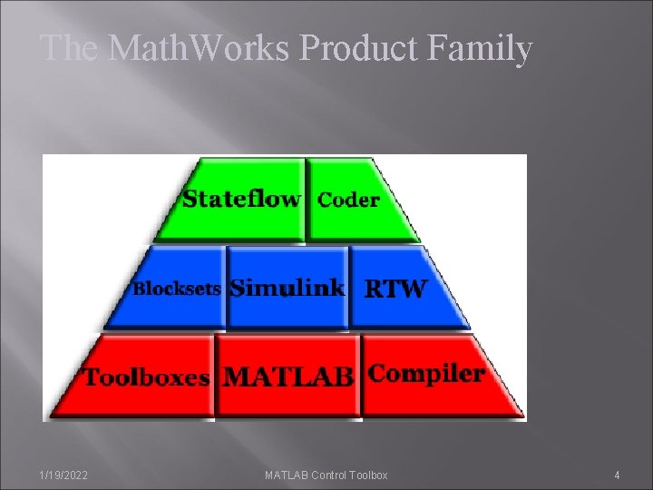
The Math. Works Product Family 1/19/2022 MATLAB Control Toolbox 4

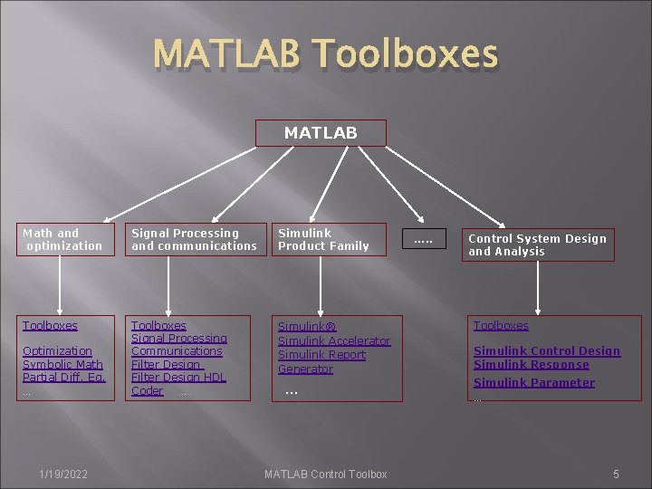
MATLAB Toolboxes MATLAB Math and optimization Signal Processing and communications Simulink Product Family Toolboxes Signal Processing Communications Filter Design HDL Coder … Simulink® Simulink Accelerator Simulink Report Generator Optimization Symbolic Math Partial Diff. Eq. … 1/19/2022 … MATLAB Control Toolbox …. . Control System Design and Analysis Toolboxes Simulink Control Design Simulink Response Simulink Parameter … 5

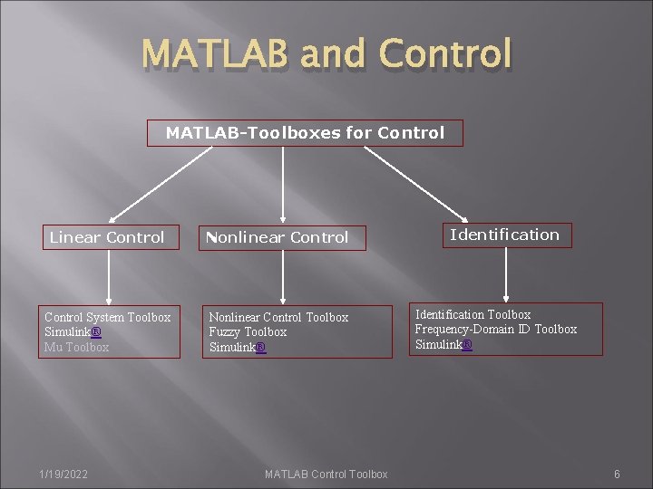
MATLAB and Control MATLAB-Toolboxes for Control Linear Control Nonlinear Control System Toolbox Simulink® Mu Toolbox Nonlinear Control Toolbox Fuzzy Toolbox Simulink® 1/19/2022 MATLAB Control Toolbox Identification Toolbox Frequency-Domain ID Toolbox Simulink® 6

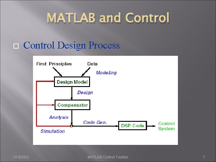
MATLAB and Control Design Process 1/19/2022 MATLAB Control Toolbox 7

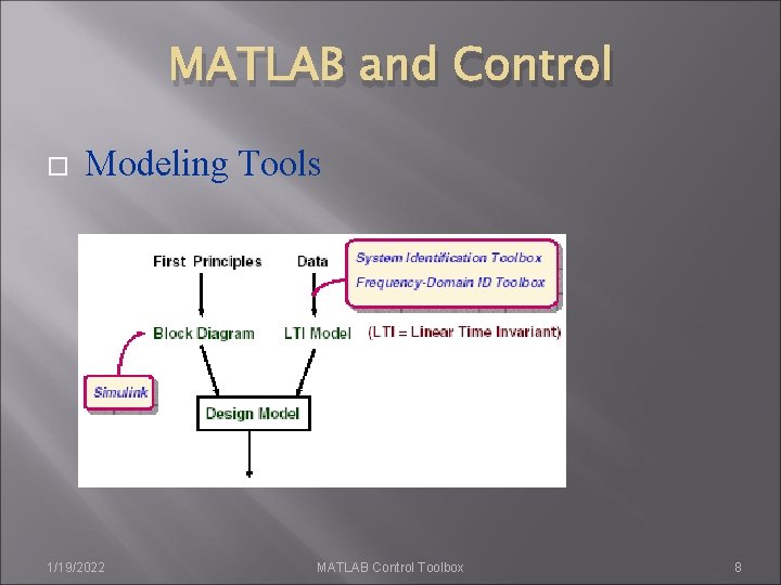
MATLAB and Control Modeling Tools 1/19/2022 MATLAB Control Toolbox 8

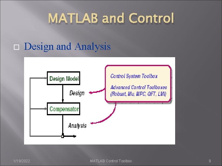
MATLAB and Control Design and Analysis 1/19/2022 MATLAB Control Toolbox 9

Control System Toolbox Core Features Tools to manipulate LTI models Classical analysis and design Bode, Nyquist, Nichols diagrams Step and impulse response Gain/phase margins Root locus design Modern state-space techniques Pole placement LQG regulation 1/19/2022 MATLAB Control Toolbox 10

Control System Toolbox LTI Objects (Linear Time Invariant) 4 basic types of LTI models Transfer Function (TF) Zero-pole-gain model (ZPK) State-Space models (SS) Frequency response data model (FRD) Conversion between models Model properties (dynamics) 1/19/2022 MATLAB Control Toolbox 11

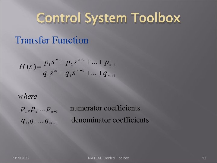
Control System Toolbox Transfer Function 1/19/2022 MATLAB Control Toolbox 12

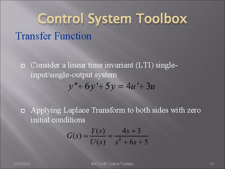
Control System Toolbox Transfer Function Consider a linear time invariant (LTI) singleinput/single-output system Applying Laplace Transform to both sides with zero initial conditions 1/19/2022 MATLAB Control Toolbox 13

Control System Toolbox Transfer Function >> num = [4 3]; >> den = [1 6 5]; >> sys = tf(num, den) Transfer function: 4 s+3 --------s^2 + 6 s + 5 1/19/2022 >> [num, den] = tfdata(sys, 'v') num = 0 4 3 den = 1 6 5 MATLAB Control Toolbox 14

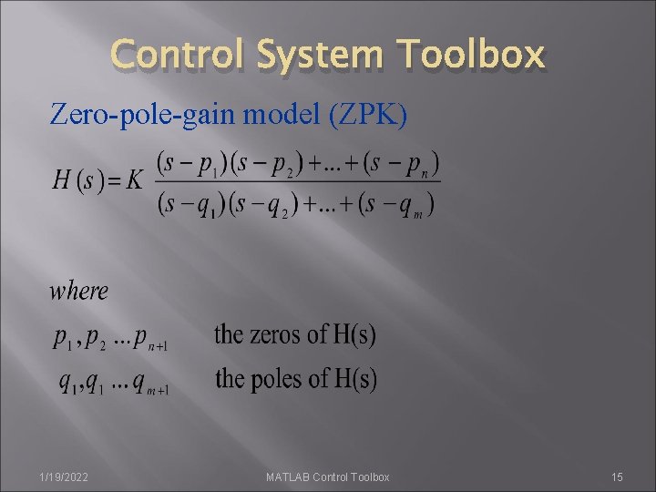
Control System Toolbox Zero-pole-gain model (ZPK) 1/19/2022 MATLAB Control Toolbox 15

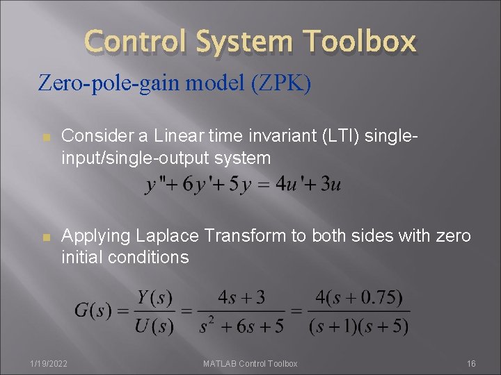
Control System Toolbox Zero-pole-gain model (ZPK) n Consider a Linear time invariant (LTI) singleinput/single-output system n Applying Laplace Transform to both sides with zero initial conditions 1/19/2022 MATLAB Control Toolbox 16

Control System Toolbox Zero-pole-gain model (ZPK) >> sys 1 = zpk(-0. 75, [-1 -5], 4) Zero/pole/gain: 4 (s+0. 75) -----(s+1) (s+5) 1/19/2022 >> [ze, po, k] = zpkdata(sys 1, 'v') ze = -0. 7500 po = -1 -5 k= 4 MATLAB Control Toolbox 17

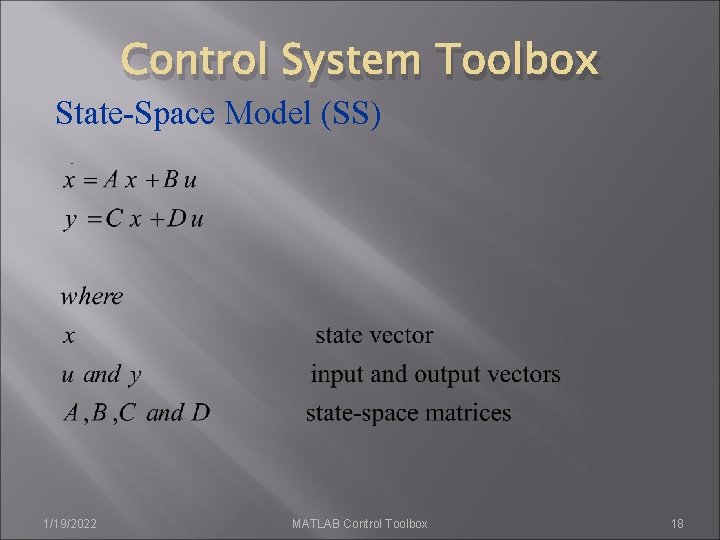
Control System Toolbox State-Space Model (SS) 1/19/2022 MATLAB Control Toolbox 18

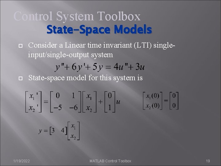
Control System Toolbox State-Space Models Consider a Linear time invariant (LTI) singleinput/single-output system State-space model for this system is 1/19/2022 MATLAB Control Toolbox 19

Control System Toolbox State-Space Models >> sys = ss([0 1; -5 -6], [0; 1], [3, 4], 0) a= x 1 x 2 x 1 0 1 x 2 -5 -6 b= u 1 x 1 0 x 2 1 1/19/2022 c= x 1 x 2 y 1 3 4 d= u 1 y 1 0 MATLAB Control Toolbox 20

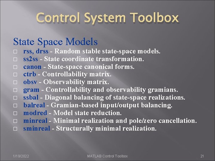
Control System Toolbox State Space Models � � � rss, drss - Random stable state-space models. ss 2 ss - State coordinate transformation. canon - State-space canonical forms. ctrb - Controllability matrix. obsv - Observability matrix. gram - Controllability and observability gramians. ssbal - Diagonal balancing of state-space realizations. balreal - Gramian-based input/output balancing. modred - Model state reduction. minreal - Minimal realization and pole/zero cancellation. sminreal - Structurally minimal realization. 1/19/2022 MATLAB Control Toolbox 21

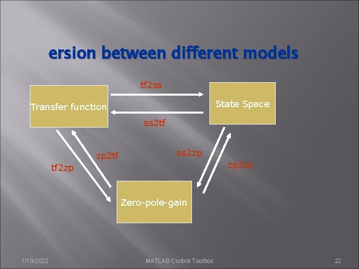
ersion between different models tf 2 ss State Space Transfer function ss 2 tf zp 2 tf ss 2 zp zp 2 ss tf 2 zp Zero-pole-gain 1/19/2022 MATLAB Control Toolbox 22

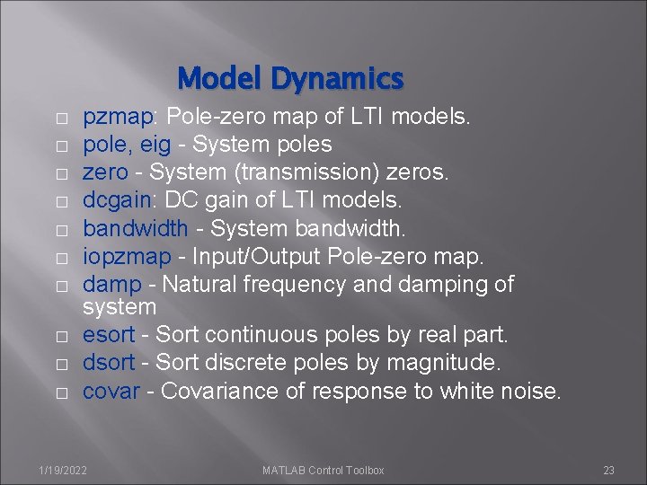
Model Dynamics � � � � � pzmap: Pole-zero map of LTI models. pole, eig - System poles zero - System (transmission) zeros. dcgain: DC gain of LTI models. bandwidth - System bandwidth. iopzmap - Input/Output Pole-zero map. damp - Natural frequency and damping of system esort - Sort continuous poles by real part. dsort - Sort discrete poles by magnitude. covar - Covariance of response to white noise. 1/19/2022 MATLAB Control Toolbox 23

Control System Toolbox Time Response of Systems 1/19/2022 Impulse Response (impulse) Step Response (step) General Time Response (lsim) Polynomial multiplication (conv) Polynomial division (deconv) Partial Fraction Expansion (residue) gensig - Generate input signal for lsim. MATLAB Control Toolbox 24

Control System Toolbox Time Response of Systems n n n The impulse response of a system is its output when the input is a unit impulse. The step response of a system is its output when the input is a unit step. The general response of a system to any input can be computed using the lsim command. 1/19/2022 MATLAB Control Toolbox 25

Control System Toolbox Time Response of Systems Problem Given the LTI system Plot the following responses for: n The impulse response using the impulse command. n The step response using the step command. n The response to the input calculated using both the lsim commands 1/19/2022 MATLAB Control Toolbox 26

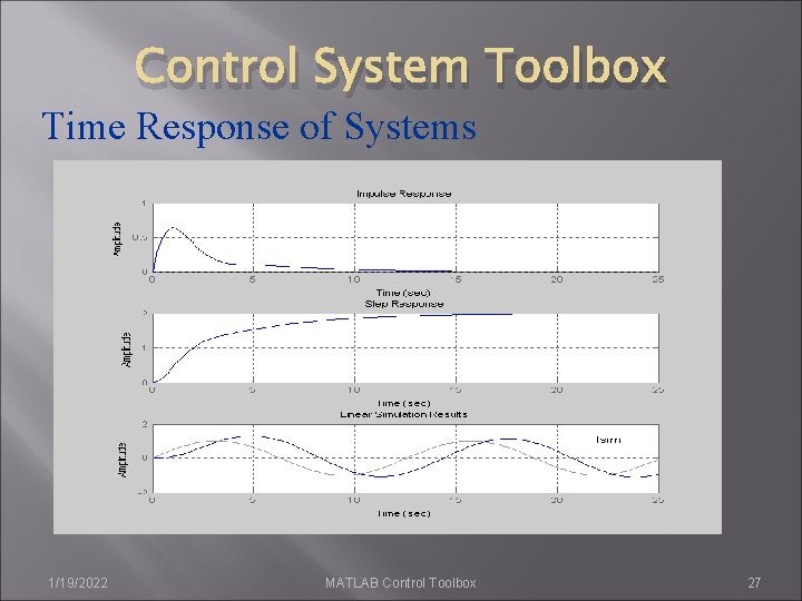
Control System Toolbox Time Response of Systems 1/19/2022 MATLAB Control Toolbox 27

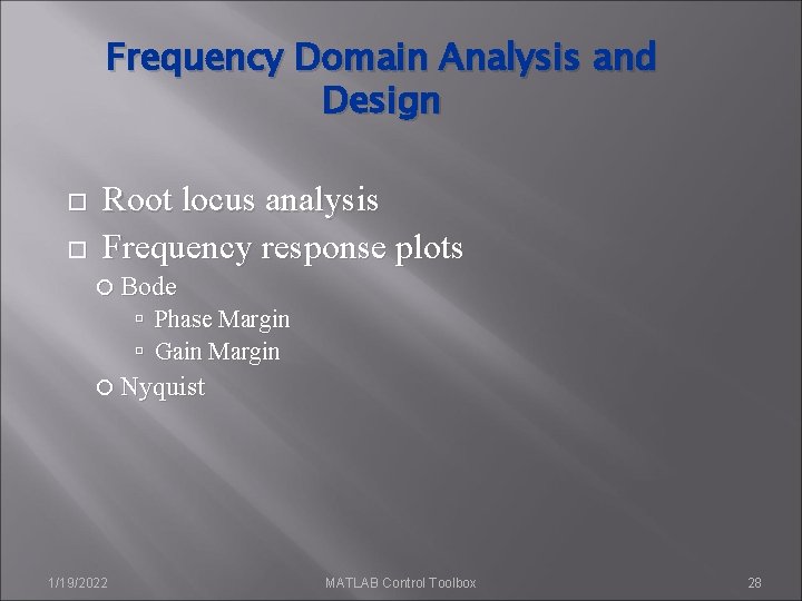
Frequency Domain Analysis and Design Root locus analysis Frequency response plots Bode Phase Margin Gain Margin Nyquist 1/19/2022 MATLAB Control Toolbox 28

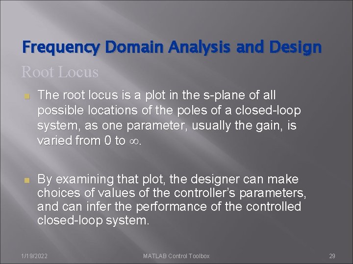
Frequency Domain Analysis and Design Root Locus n The root locus is a plot in the s-plane of all possible locations of the poles of a closed-loop system, as one parameter, usually the gain, is varied from 0 to . n By examining that plot, the designer can make choices of values of the controller’s parameters, and can infer the performance of the controlled closed-loop system. 1/19/2022 MATLAB Control Toolbox 29

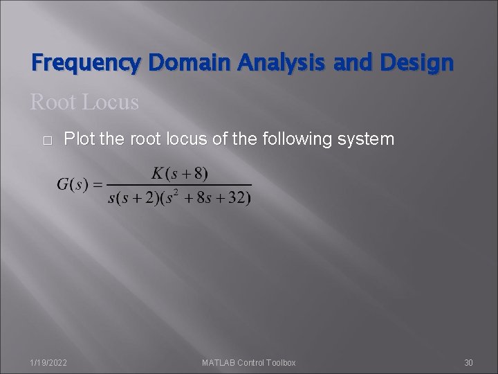
Frequency Domain Analysis and Design Root Locus � Plot the root locus of the following system 1/19/2022 MATLAB Control Toolbox 30

Frequency Domain Analysis and Design Root Locus >> rlocus(tf([1 8], conv([1 0], [1 2]), [1 8 32]))) 1/19/2022 MATLAB Control Toolbox 31

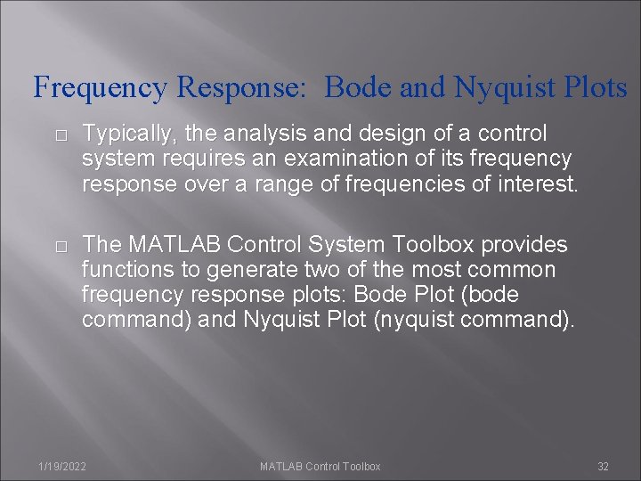
Frequency Response: Bode and Nyquist Plots � Typically, the analysis and design of a control system requires an examination of its frequency response over a range of frequencies of interest. � The MATLAB Control System Toolbox provides functions to generate two of the most common frequency response plots: Bode Plot (bode command) and Nyquist Plot (nyquist command). 1/19/2022 MATLAB Control Toolbox 32

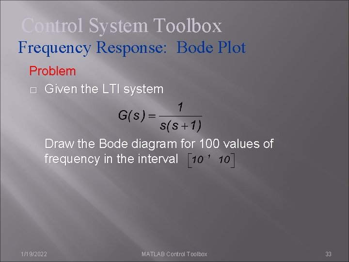
Control System Toolbox Frequency Response: Bode Plot Problem � Given the LTI system Draw the Bode diagram for 100 values of frequency in the interval. 1/19/2022 MATLAB Control Toolbox 33

Control System Toolbox Frequency Response: Bode Plot >>bode(tf(1, [1 1 0]), logspace(-1, 1, 100)); 1/19/2022 MATLAB Control Toolbox 34

Control System Toolbox Frequency Response: Nyquist Plot n n n The loop gain Transfer function G(s) The gain margin is defined as the multiplicative amount that the magnitude of G(s) can be increased before the closed loop system goes unstable Phase margin is defined as the amount of additional phase lag that can be associated with G(s) before the closed-loop system goes unstable 1/19/2022 MATLAB Control Toolbox 35

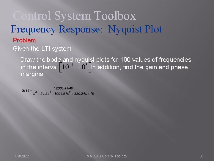
Control System Toolbox Frequency Response: Nyquist Plot Problem Given the LTI system Draw the bode and nyquist plots for 100 values of frequencies in the interval. In addition, find the gain and phase margins. 1/19/2022 MATLAB Control Toolbox 36

Control System Toolbox Frequency Response: Nyquist Plot w=logspace(-4, 3, 100); sys=tf([1280 640], [1 24. 2 1604. 81 320. 24 16]); bode(sys, w) [Gm, Pm, Wcg, Wcp]=margin(sys) %Nyquist plot figure nyquist(sys, w) 1/19/2022 MATLAB Control Toolbox 37

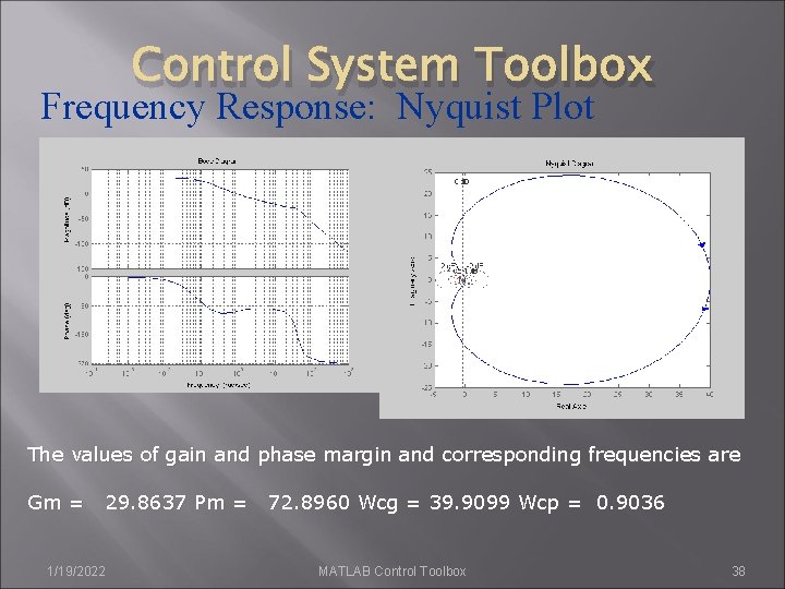
Control System Toolbox Frequency Response: Nyquist Plot The values of gain and phase margin and corresponding frequencies are Gm = 1/19/2022 29. 8637 Pm = 72. 8960 Wcg = 39. 9099 Wcp = 0. 9036 MATLAB Control Toolbox 38

Frequency Response Plots bode - Bode diagrams of the frequency response. bodemag - Bode magnitude diagram only. sigma - Singular value frequency plot. Nyquist - Nyquist plot. nichols - Nichols plot. margin - Gain and phase margins. allmargin - All crossover frequencies and related gain/phase margins. freqresp - Frequency response over a frequency grid. evalfr - Evaluate frequency response at given frequency. interp - Interpolates frequency response data. Control System Toolbox 1/19/2022 MATLAB Control Toolbox 39

Control System Toolbox Design: Pole Placement � � place - MIMO pole placement. acker - SISO pole placement. estim - Form estimator given estimator gain. reg - Form regulator given state-feedback and estimator gains. 1/19/2022 MATLAB Control Toolbox 40

Control System Toolbox Design : LQR/LQG design � � � � lqr, dlqr - Linear-quadratic (LQ) state-feedback regulator. lqry - LQ regulator with output weighting. lqrd - Discrete LQ regulator for continuous plant. kalman - Kalman estimator. kalmd - Discrete Kalman estimator for continuous plant. lqgreg - Form LQG regulator given LQ gain and Kalman estimator. augstate - Augment output by appending states. 1/19/2022 MATLAB Control Toolbox 41

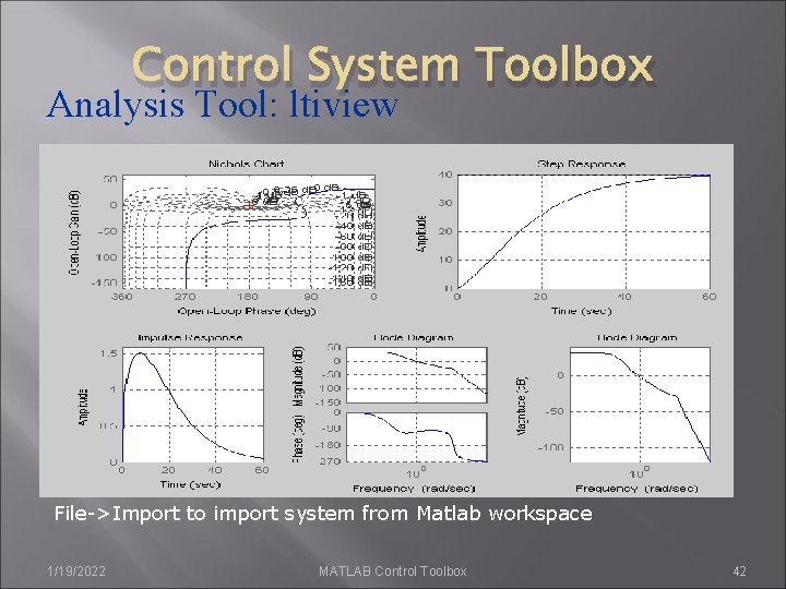
Control System Toolbox Analysis Tool: ltiview File->Import to import system from Matlab workspace 1/19/2022 MATLAB Control Toolbox 42

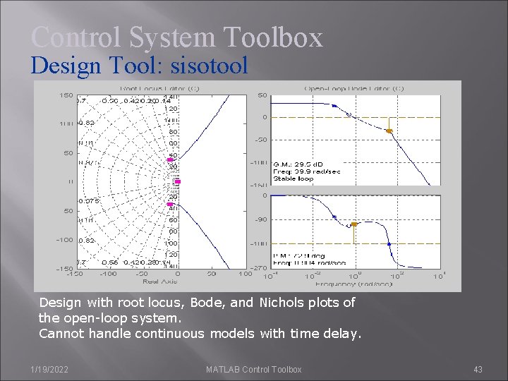
Control System Toolbox Design Tool: sisotool Design with root locus, Bode, and Nichols plots of the open-loop system. Cannot handle continuous models with time delay. 1/19/2022 MATLAB Control Toolbox 43

M-File Example %Define the transfer function of a plant G=tf([4 3], [1 6 5]) %find the bandwidth of the new system wb=bandwidth(T) %Get data from the transfer function [n, d]=tfdata(G, 'v') %plot the step response step(T) [p, z, k]=zpkdata(G, 'v') %plot the rootlocus rlocus(T) [a, b, c, d]=ssdata(G) %Check the controllability and observability of the system ro=rank(obsv(a, c)) rc=rank(ctrb(a, b)) %obtain the bode plots bode(T) margin(T) %find the eigenvalues of the system damp(a) %use the LTI viewer ltiview({'step'; 'bode'; 'nyquist'}, T) %multiply the transfer function with another transfer function T=series(G, zpk([-1], [-10 -2 j +2 j], 5)) %start the SISO tool sisotool(T) %plot the poles and zeros of the new system iopzmap(T) 1/19/2022 MATLAB Control Toolbox 44