Mathematics Statistics Topic 3 Describing Data Numerical Topic

Mathematics & Statistics Topic 3 Describing Data: Numerical

Topic Goals After completing this topic, you should be able to: n n Compute and interpret the mean, median, and mode for a set of data Find the range, variance, standard deviation, and coefficient of variation and know what these values mean Apply the empirical rule to describe the variation of population values around the mean Explain how covariance and correlation measure a linear relationship between two variables

Describing Data Numerically Central Tendency Variation Arithmetic Mean Range Median Interquartile Range Mode Variance Standard Deviation Coefficient of Variation

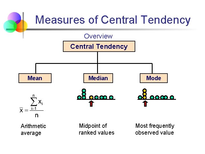
Measures of Central Tendency Overview Central Tendency Mean Median Mode Arithmetic average Midpoint of ranked values Most frequently observed value

Arithmetic Mean n The arithmetic mean (mean) is the most common measure of central tendency n For a population of N values: Population values Population size n For a sample of size n: Observed values Sample size

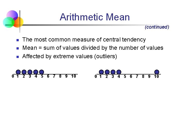
Arithmetic Mean (continued) n n n The most common measure of central tendency Mean = sum of values divided by the number of values Affected by extreme values (outliers) 0 1 2 3 4 5 6 7 8 9 10

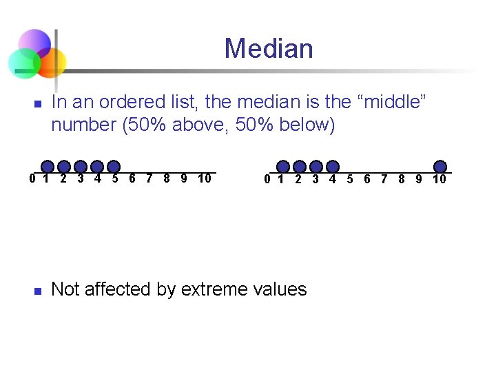
Median n In an ordered list, the median is the “middle” number (50% above, 50% below) 0 1 2 3 4 5 6 7 8 9 10 n 0 1 2 3 4 5 6 7 8 9 10 Not affected by extreme values

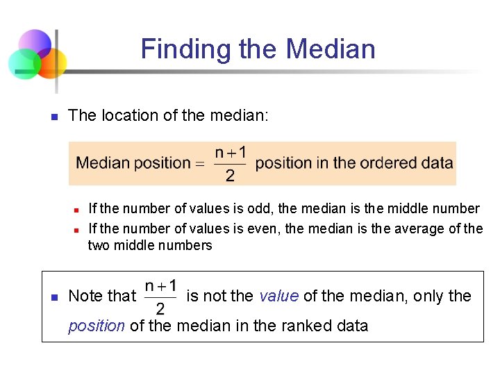
Finding the Median n The location of the median: n n n If the number of values is odd, the median is the middle number If the number of values is even, the median is the average of the two middle numbers Note that is not the value of the median, only the position of the median in the ranked data

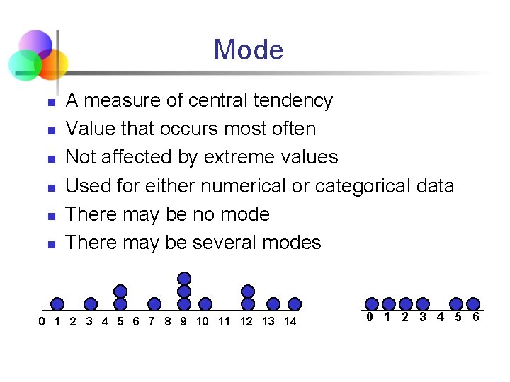
Mode n n n A measure of central tendency Value that occurs most often Not affected by extreme values Used for either numerical or categorical data There may be no mode There may be several modes 0 1 2 3 4 5 6 7 8 9 10 11 12 13 14 0 1 2 3 4 5 6

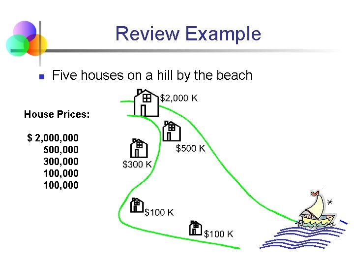
Review Example n Five houses on a hill by the beach House Prices: $ 2, 000 500, 000 300, 000 100, 000

Which measure of location is the “best”? n Mean is generally used, unless extreme values (outliers) exist n n We will use the mean extensively in later topics. Always ask yourself: Is it the mean I am interested in? Then median is often used, since the median is not sensitive to extreme values. n Example: Median home prices may be reported for a region – less sensitive to outliers

Shape of a Distribution n Describes how data are distributed n Measures of shape n Symmetric or skewed (mean vs median)

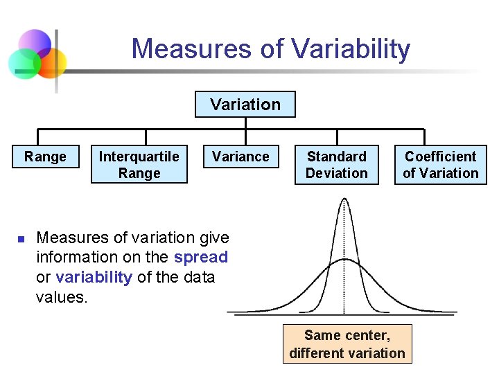
Measures of Variability Variation Range n Interquartile Range Variance Standard Deviation Coefficient of Variation Measures of variation give information on the spread or variability of the data values. Same center, different variation

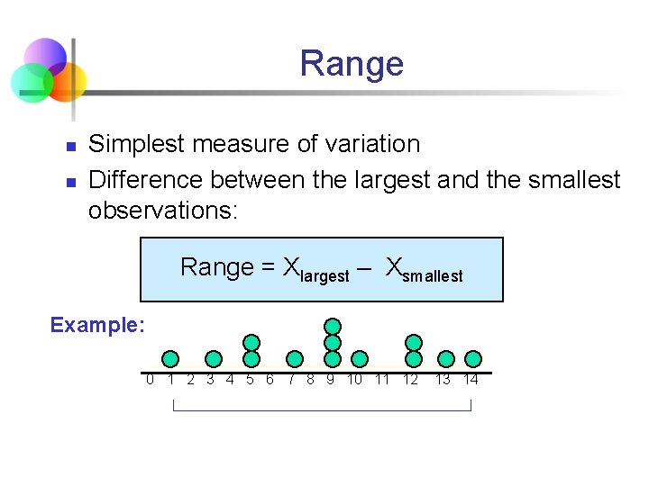
Range n n Simplest measure of variation Difference between the largest and the smallest observations: Range = Xlargest – Xsmallest Example: 0 1 2 3 4 5 6 7 8 9 10 11 12 13 14

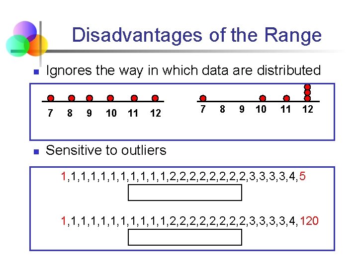
Disadvantages of the Range n Ignores the way in which data are distributed 7 n 8 9 10 11 12 7 8 9 10 11 12 Sensitive to outliers 1, 1, 1, 2, 2, 3, 3, 4, 5 1, 1, 1, 2, 2, 3, 3, 4, 120

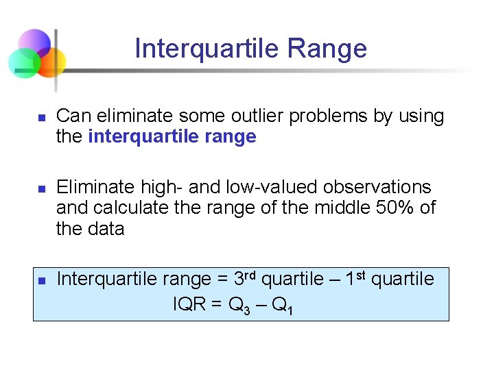
Interquartile Range n n n Can eliminate some outlier problems by using the interquartile range Eliminate high- and low-valued observations and calculate the range of the middle 50% of the data Interquartile range = 3 rd quartile – 1 st quartile IQR = Q 3 – Q 1

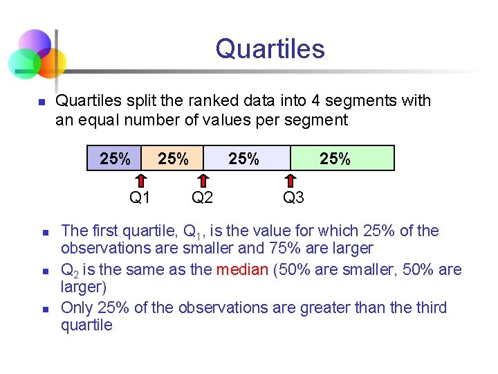
Quartiles n Quartiles split the ranked data into 4 segments with an equal number of values per segment 25% Q 1 n n n 25% Q 2 25% Q 3 The first quartile, Q 1, is the value for which 25% of the observations are smaller and 75% are larger Q 2 is the same as the median (50% are smaller, 50% are larger) Only 25% of the observations are greater than the third quartile

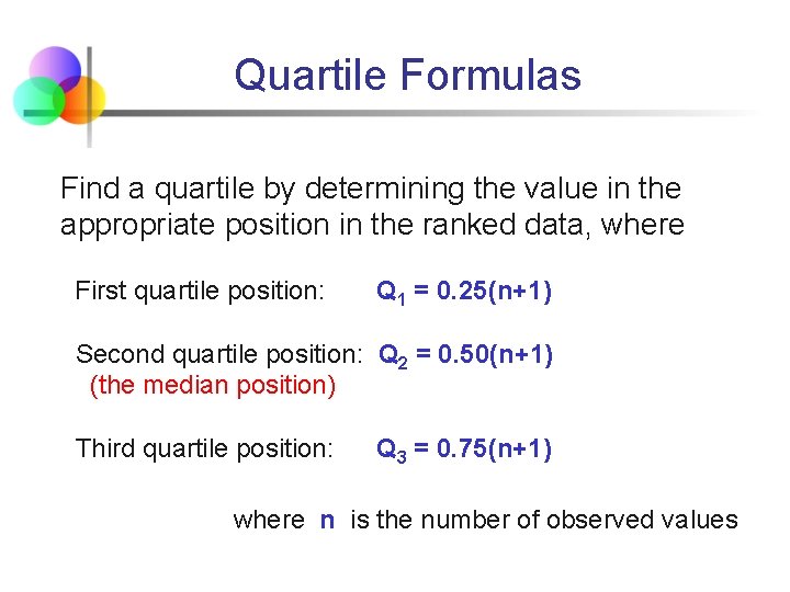
Quartile Formulas Find a quartile by determining the value in the appropriate position in the ranked data, where First quartile position: Q 1 = 0. 25(n+1) Second quartile position: Q 2 = 0. 50(n+1) (the median position) Third quartile position: Q 3 = 0. 75(n+1) where n is the number of observed values

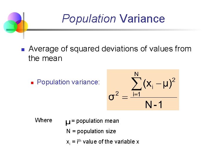
Population Variance n Average of squared deviations of values from the mean n Population variance: Where = population mean N = population size xi = ith value of the variable x

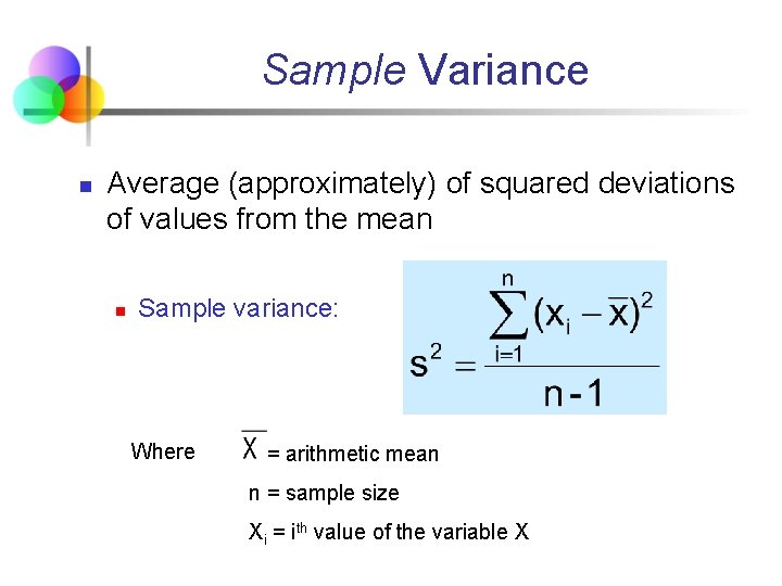
Sample Variance n Average (approximately) of squared deviations of values from the mean n Sample variance: Where = arithmetic mean n = sample size Xi = ith value of the variable X

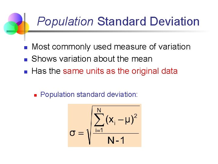
Population Standard Deviation n Most commonly used measure of variation Shows variation about the mean Has the same units as the original data n Population standard deviation:

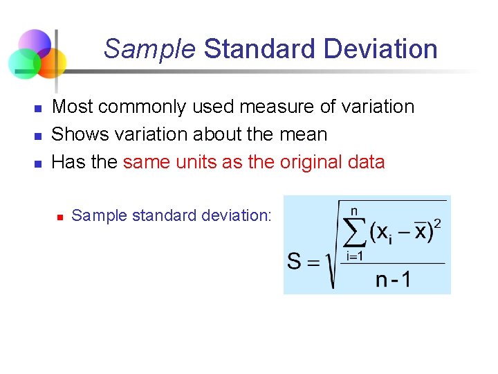
Sample Standard Deviation n Most commonly used measure of variation Shows variation about the mean Has the same units as the original data n Sample standard deviation:

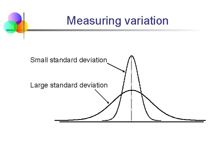
Measuring variation Small standard deviation Large standard deviation

Comparing Standard Deviations Data A 11 12 13 14 15 16 17 18 19 20 21 Data B 11 12 Data C 11 12 13

Advantages of Variance and Standard Deviation n n Each value in the data set is used in the calculation Values far from the mean are given extra weight (because deviations from the mean are squared)

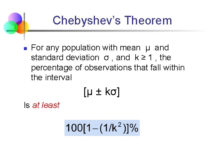
Chebyshev’s Theorem n For any population with mean μ and standard deviation σ , and k ≥ 1 , the percentage of observations that fall within the interval [μ ± kσ] Is at least

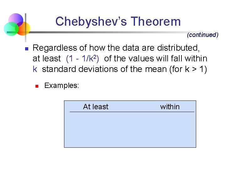
Chebyshev’s Theorem (continued) n Regardless of how the data are distributed, at least (1 - 1/k 2) of the values will fall within k standard deviations of the mean (for k > 1) n Examples: At least within

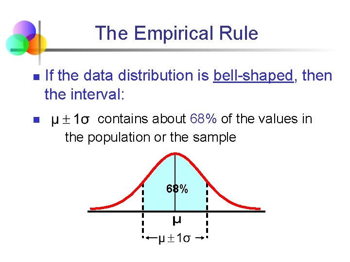
The Empirical Rule n n If the data distribution is bell-shaped, then the interval: contains about 68% of the values in the population or the sample 68%

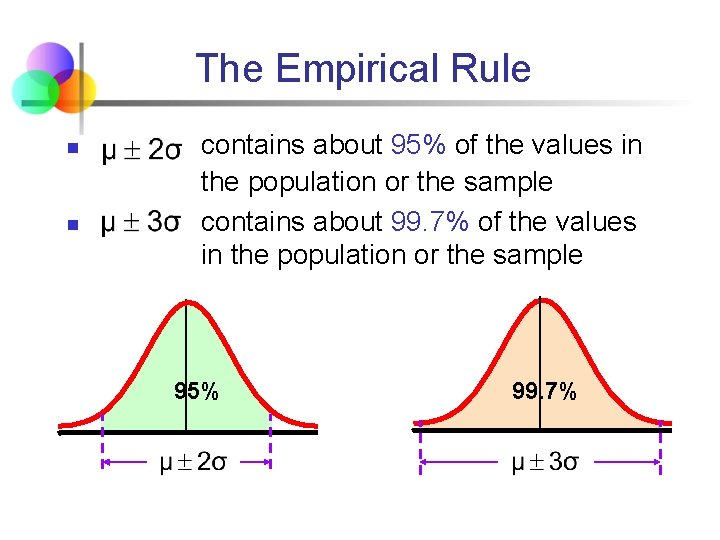
The Empirical Rule n n contains about 95% of the values in the population or the sample contains about 99. 7% of the values in the population or the sample 95% 99. 7%

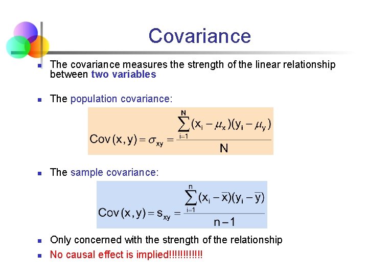
Covariance n The covariance measures the strength of the linear relationship between two variables n The population covariance: n The sample covariance: n n Only concerned with the strength of the relationship No causal effect is implied!!!!!!

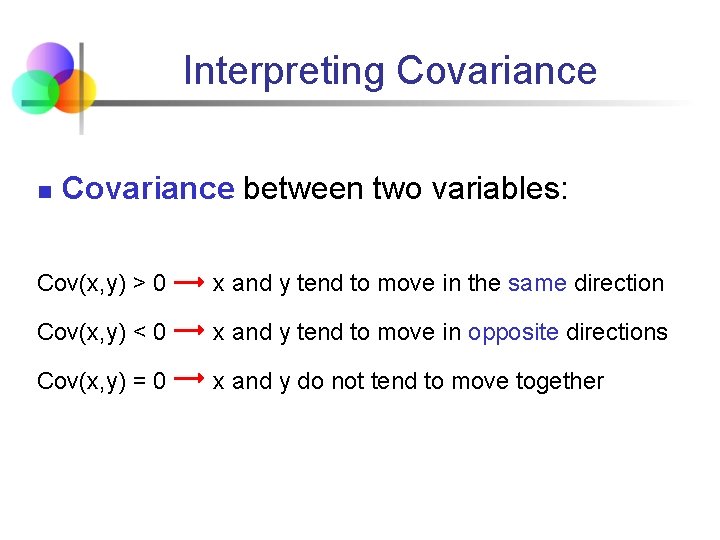
Interpreting Covariance n Covariance between two variables: Cov(x, y) > 0 x and y tend to move in the same direction Cov(x, y) < 0 x and y tend to move in opposite directions Cov(x, y) = 0 x and y do not tend to move together

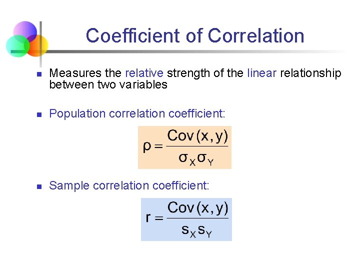
Coefficient of Correlation n Measures the relative strength of the linear relationship between two variables n Population correlation coefficient: n Sample correlation coefficient:

Features of Correlation Coefficient, r n Unit free n Ranges between – 1 and 1 n n The closer to – 1, the stronger the negative linear relationship The closer to 1, the stronger the positive linear relationship The closer to 0, the weaker any linear relationship Related to “best-fitting” straight line through scatter plot (linear regression)

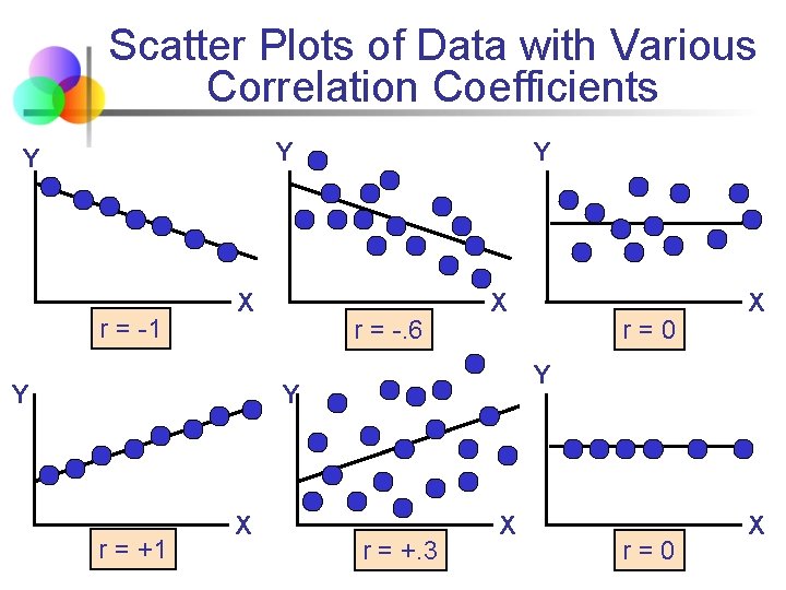
Scatter Plots of Data with Various Correlation Coefficients Y Y r = -1 X Y Y r = -. 6 X Y Y r = +1 X r=0 X r = +. 3 X r=0 X

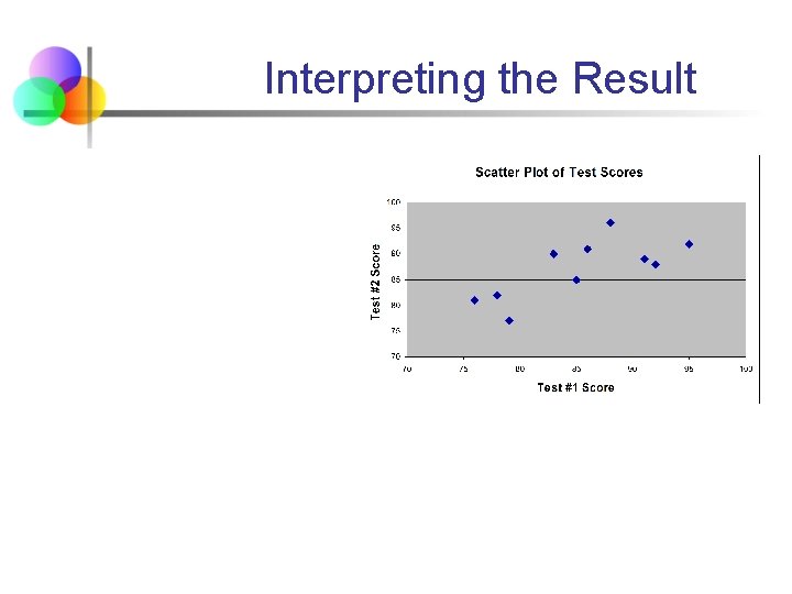
Interpreting the Result

Topic Summary n Described measures of central tendency n n Illustrated the shape of the distribution n n Symmetric, skewed Described measures of variation n n Mean, median, mode Range, interquartile range, variance and standard deviation, coefficient of variation Calculated measures of relationships between variables n covariance and correlation coefficient