Mathematics IV Complex Variables and Fourier Analysis By

Mathematics IV (Complex Variables and Fourier Analysis) By M. AMARNATH Assistant Professor, Department of Humanities & Sciences K. G. Reddy College of Engineering and Technology 2018 -2019

Unit-I Functions of a Complex Variable

Complex number: Complex algebra: Complex conjugation: Polar representation: Modulus (magnitude): Argument (phase): 3

Complex Function Definition. Complex function of a complex variable. Let C. A function f defined on is a rule which assigns to each z a complex number w. The number w is called a value of f at z and is denoted by f(z), i. e. , w = f(z). The set is called the domain of definition of f. Although the domain of definition is often a domain, it need not be. 4

Remark Properties of a real-valued function of a real variable are often exhibited by the graph of the function. But when w = f(z), where z and w are complex, no such convenient graphical representation is available because each of the numbers z and w is located in a plane rather than a line. We can display some information about the function by indicating pairs of corresponding points z = (x , y) and w = ( u, v). To do this, it is usually easiest to draw the z and w planes separately. 5

Graph of Complex Function y w = f(z) v x u domain of definition zplane range w-plane 6

Example 1 Describe the range of the function f(z) = x 2 + 2 i, defined on (the domain is) the unit disk |z| 1. Solution: We have u( x, y) = x 2 and v( x, y) = 2. Thus as z varies over the closed unit disk, u varies between 0 and 1, and v is constant (=2). Therefore w = f(z) = u(x , y ) + iv( x, y) = x 2 +2 i is a line segment from w = 2 i to w = 1 + 2 i. y domain f(z) x v range u 7

Functions of a complex variable: All elementary functions of real variables may be extended into the complex plane. A complex function can be resolved into its real part and imaginary part: Multi-valued functions and branch cuts: To remove the ambiguity, we can limit all phases to (- p, p). q = -p is the branch cut. lnz with n = 0 is the principle value. We can let z move on 2 Riemann sheets so that is single valued everywhere. 8

Cauchy-Riemann conditions Analytic functions: If f (z) is differentiable at z = z 0 and within the neighborhood of z=z 0, f (z) is said to be analytic at z = z 0. A function that is analytic in the whole complex plane is called an entire function. Cauchy-Riemann conditions for differentiability In order to let f be differentiable, f '(z) must be the same in any direction of z. Particularly , it is necessary that Cauchy-Riemann conditions 9

Conversely, if the Cauchy-Riemann conditions are satisfied, f (z) is differentiable: More about Cauchy-Riemann conditions: 1) It is a very strong restraint to functions of a complex variable. 2) 3) 4) 10

General search for Cauchy-Riemann conditions: Our Cauchy-Riemann conditions were derived by requiring f '(z) be the same when z changes along x or y directions. How about other directions? Here I do a general search for the conditions of differentiability. 11

Harmonic Functions • Definition. Harmonic. A real-valued function (x , y ) is said to be harmonic in a domain D if all of its second-order partial derivatives are continuous in D and if each point of D satisfies Theorem: If f (z) = u( x, y) + iv( x, y) is analytic in a domain D, then each of the functions u(x , y) and v(x , y) is harmonic in D. 12

Harmonic Conjugate Given a function u(x , y) harmonic in, say, an open disk, then we can find another harmonic function v(x , y) so that u + iv is an analytic function of z in the disk. Such a function v is called a harmonic conjugate of u. Example Construct an analytic function whose real part is: Solution: First verify that this function is harmonic 13

Example, Continued 14

Example, Continued Integrate (1) with respect to y: Now take the derivative of v( x, y) with respect to x: 15

Example, Continued According to equation (2), this equals 6 xy – 1. Thus, 16

Example, Continued The desired analytic function f (z) = u + iv is: Thank you 17

Unit II Complex integration and power series

Contour integral: Cauchy’s integral theorem: If f (z) is analytic in a simply connected region R, [and f ′(z) is continuous throughout this region, ] then for any closed path C in R, the contour integral of f (z) around C is zero: Proof using Stokes’ theorem: 19

Cauchy-Goursat proof: The continuity of f '(z) is not necessary. z 2 Corollary: An open contour integral for an analytic function is independent of the path, if there is no singular points between the paths. z 1 Contour deformation theorem: A contour of a complex integral can be arbitrarily deformed through an analytic region without changing the integral. C 2 1) It applies to both open and closed contours. 2) One can even split closed contours. Proof: Deform the contour bit by bit. Examples: 1) Cauchy’s integral theorem. (Let the contour shrink to a point. ) 2) Cauchy’s integral formula. (Let the contour shrink to a small circle. ) z 2 “nails” z 1 C 1 “rubber bands” C 2 C 1 C 3 C 1 20

Cauchy’s integral formula: If f (z) is analytic within and on a closed contour C, then for any point z 0 within C, L 1 z 0 L 2 C 0 C Can directly use the contour deformation theorem. 21

Derivatives of f (z): Corollary: If a function is analytic, then its derivatives of all orders exist. Corollary: If a function is analytic, then it can be expanded in Taylor series. Cauchy’s inequality: If is analytic and bounded, then Liouville’s theorem: If a function is analytic and bounded in the entire complex plane, then this function is a constant. Fundamental theorem of algebra: has n roots. Suppose P(z) has no roots, then 1/P(z) is analytic and bounded as nonsense. Therefore P(z) has at least one root we can divide out. Then P(z) is constant. That is 22

Morera’s theorem: If f (z) is continuous and connected region, then f (z) is analytic in this region. for every closed contour within a simply 23

Analytic continuation Laurent expansion Taylor expansion for functions of a complex variable: Expanding an analytic function f (z) about z = z 0, where z 1 is the nearest singular point. z 24

Analytic continuation: Suppose f (z) is analytic around z = z 0, we can expand it about z = z 0 in a Taylor series: This series converges inside a circle with a radius of convergence , where a 0 is the nearest singularity from z = z 0. We can also expand f (z) about another point z = z 1 within the circle R 0: z 0 . In general, the new circle has a radius of convergence circle. a 0 R 0 z 1 and contains points not within the first a 1 R 1 Consequences: 1) f (z) can be analytically continued over the complex plane, excluding singularities. 2) If f (z) is analytic, its values at one region determines its values everywhere. 25

Laurent expansion Problem: Expanding a function f (z) that is analytic in an annular region (between r and R). L 2 L 1 C is any contour that encloses z 0 and lies between r and R (deformation theorem). 26

Laurent expansion: 1) 2) 3) Singular points of the integrand. For n < 0, the singular points are determined by f (z). For n ≥ 0, the singular points are determined by both f (z) and 1/(z'-z 0)n+1. If f (z) is analytic inside C, then the Laurent series reduces to a Taylor series: Although an has a general contour integral form, In most times we need to use straight forward complex algebra to find an. 27

Laurent expansion: Examples Example 1: Expand Example 2: Expand about z 0=1. about z 0=i. 28

Branch points and branch cuts Singularities Poles: In a Laurent expansion then z 0 is said to be a pole of order n. A pole of order 1 is called a simple pole. A pole of infinite order (when expanded about z 0) is called an essential singularity. The behavior of a function f (z) at infinity is defined using the behavior of f (1/t) at t = 0. Examples: sinz thus has an essential singularity at infinity. 29

Residue theorem Calculus of residues Suppose an analytic function f (z) has an isolated singularity at z 0. Consider a contour integral enclosing z 0 The coefficient a-1=Res f (z 0) in the Laurent expansion is called the residue of f (z) at z = z 0. If the contour encloses multiple isolated singularities, we have the residue theorem: z 0 z 1 Contour integral =2 pi ×Sum of the residues at the enclosed singular points 30 30

Residue formula: To find a residue, we need to do the Laurent expansion and pick up the coefficient a-1. However, in many cases we have a useful residue formula 31 31

32

33 33

Unit III Evaluation of definite integrals and Bilinear transformation

L’Hospital’s rule: 35 35

I. Integrals of trigonometric functions : C r=1 36

z- z+ C r=1 37

z- z+ C r=1 38

z+ zz 0 C r=1 39

Evaluation of definite integrals -2 II. Integrals along the whole real axis: Assumption 1: f (z) is analytic in the upper or lower half of the complex plane, except isolated finite number of poles. Condition for closure on a semicircular path: ∩ R Assumption 2: when |z| & | f (z)| goes to zero faster than 1/|z|. Then, 40

41

III. Fourier integrals: Assumption 1: f (z) is analytic in the upper half of the complex plane, except isolated finite number of poles. ∩ Jordan’s lemma: R 42

Question: How about Answer: We can go the lower half of the complex plane using a clockwise contour. 43

Question: How about Answer: 44

45

46

47

48

49

Unit IV Fourier Series and Fourier Transform

Introduction � Any function of a variable, whether continuous or discontinuous, can be expanded in a series of sines of multiples of the variable. � Fourier series is very useful in solving ordinary and partial differential equation.

� Even, Odd, and Periodic Functions

Fourier Series of a Periodic Function Definition : A Fourier series may be defined as an expansion of a� function in a series of sines and cosines such as , The coefficients are related to the periodic function f(x) by definite integrals: Henceforth we assume f satisfies the following (Dirichlet) conditions: (1) f(x) is a periodic function; (2) f(x) has only a finite number of finite discontinuities; (3) f(x) has only a finite number of extrem values, maxima and minima in the interval [0, 2 p].

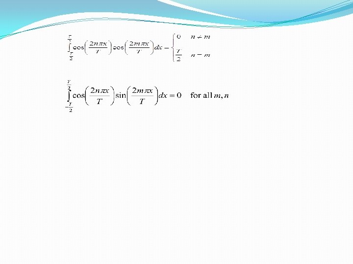
EULER’S FORMULA The formula for a Fourier series is: N We have formulae for the coefficients (for the derivations see the course notes): One very important property of sines and cosines is their orthogonality, expressed by:

Summary of finding coefficients function even Though maybe easy to find using geometry function odd function neither Though maybe easy to find using geometry

Half range Expansions It often happens in applications, especially when we solve partial differential equations by the method of separation of variables, that we need to expand a given function f in a Fourier series, where f is defined only on a finite interval. We define an “extended function”, say fext, so that fext is periodic in the domain of -∞< x < ∞, and fext=f(x) on the original interval 0<x<L. There can be infinite number of such extensions. Four extensions: half- and quarter- range cosine and sine extensions, which are based on symmetry or antisymmetry about the endpoints x=0 and x=L.

Fourier Integral If f(x) and f’(x) are piecewise continuous in every finite interval, and f(x) is absolutely integrable on R, i. e. converges, then

DIFFERENT FORMS OF FOURIER INTEGRAL THEOREM

INFINITE FOURIER TRANSFORM

Fourier Sine Transform

Properties of Fourier transform 1 Linearity: For any constants a, b the following equality holds: 2 Scaling: For any constant c, the following equality holds: 62

3. Time shifting: proof: 4. Frequency shifting: Proof:

Thank you 64

Unit V Applications of PDE

Contens The Wave Equation of Vibrating String Solution of the Wave Equation Discrete Time Traveling Wave

1 D Wave Equation u u(x, t) = ? Boundary Conditions: Initial Conditions: 0 l

Separation of Variables Assume function of t function of x constant why?

Separation of Variables F(x) = ? Boundary Conditions: F(0) = 0, F(l) =0 >0 Three Cases: k = 0 <0

k=0 F(x) = ? Boundary Conditions: F(0) = 0, F(l) =0 a = 0 and b = 0

k 2 = (>0) F(x) = ? Boundary Conditions: F(0) = 0, F(l) =0 A=0 B=0

k= 2 p (<0) F(x) = ? Boundary Conditions: F(0) = 0, F(l) =0

k= 2 p (<0)

Objectives of conduction analysis • To determine the temperature field, T(x, y, z, t), in a body • (i. e. how temperature varies with position within the body) q T(x, y, z, t) depends on: • - boundary conditions T(x, y, z) • - initial condition • - material properties (k, cp, …) • - geometry of the body (shape, size) q Why we need T(x, y, z, t) ? • - to compute heat flux at any location (using Fourier’s eqn. ) • - compute thermal stresses, expansion, deflection due to temp. etc. • - design insulation thickness • - chip temperature calculation • - heat treatment of metals

Unidirectional heat conduction (1 D) Area = A 0 Solid bar, insulated on all long sides (1 D heat conduction) qx x x+ x x A = Internal heat generation per unit vol. (W/m 3) qx+ x

Unidirectional heat conduction (1 D)(contd…) ¶T ¶T ¶ æ ¶T ö ¶T - k. A + A ç k = r Ac x ÷ x + A xq& ¶x ¶x ¶x è ¶x ø ¶t ¶ æ ¶T ö ¶T = r c çk ÷ + q& ¶x è ¶x ø ¶t Longitudinal conduction If k is a constant Internal heat generation Thermal inertia ¶ 2 T q& r c ¶T 1 ¶T + = = 2 ¶x k k ¶t a ¶t

Unidirectional heat conduction (1 D)(contd…) q For T to rise, LHS must be positive (heat input is positive) q For a fixed heat input, T rises faster for higher q In this special case, heat flow is 1 D. If sides were not insulated, heat flow could be 2 D, 3 D.

Boundary and Initial conditions: q The objective of deriving the heat diffusion equation is to determine the temperature distribution within the conducting body. q We have set up a differential equation, with T as the dependent variable. The solution will give us T(x, y, z). Solution depends on boundary conditions (BC) and initial conditions (IC).

Boundary and Initial conditions (contd…) How many BC’s and IC’s ? - Heat equation is second order in spatial coordinate. Hence, 2 BC’s needed for each coordinate. * 1 D problem: 2 BC in x-direction * 2 D problem: 2 BC in x-direction, 2 in y-direction * 3 D problem: 2 in x-dir. , 2 in y-dir. , and 2 in z-dir. - Heat equation is first order in time. Hence one IC needed