Mathematics 3 Statistics Chapter 1 DESCRIPTIVE STATISTICS PART

Mathematics 3 – Statistics Chapter 1: DESCRIPTIVE STATISTICS – PART I

What is Statistics? � Statistics is the science of learning from data exhibiting random fluctuation. � Descriptive statistics: § Collecting data § Presenting data § Describing data � Inferential statistics: § Drawing conclusions and/or making decisions concerning a population based only on sample data § Based on probability theory Chapter 1: DESCRIPTIVE STATISTICS – PART I 2

Data Presentation � What are data? § Data can be numbers, record names, or other labels. § Data are useless without their context… § To provide context we need Who, What (and in what units), When, Where, and How of the data. � In civil engineering we meet most often numerical data. � Presentation tools for numerical data (one sample): § Histogram § Boxplot Chapter 1: DESCRIPTIVE STATISTICS – PART I 3

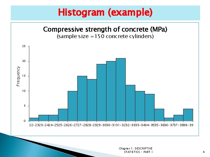
Histogram (example) Compressive strength of concrete (MPa) (sample size =150 concrete cylinders) 25 Frequency 20 15 10 5 0 22 -2323 -2424 -2525 -2626 -2727 -2828 -2929 -3030 -3131 -3232 -3333 -3434 -3535 -3636 -3737 -3838 -39 Chapter 1: DESCRIPTIVE STATISTICS – PART I 4

Data Presentation (continued) � Other examples of histograms: Example 1. 1, part a) on my personal website: mat. fsv. cvut. cz/Hala/ � How to construct a boxplot? Will be discussed later (the use of numerical measures is necessary). Chapter 1: DESCRIPTIVE STATISTICS – PART I 5

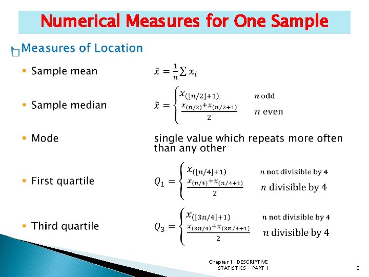
Numerical Measures for One Sample � Chapter 1: DESCRIPTIVE STATISTICS – PART I 6

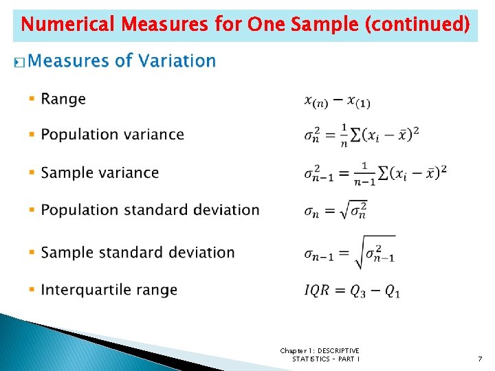
Numerical Measures for One Sample (continued) � Chapter 1: DESCRIPTIVE STATISTICS – PART I 7

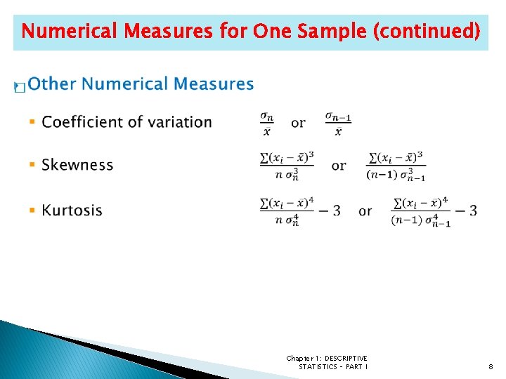
Numerical Measures for One Sample (continued) � Chapter 1: DESCRIPTIVE STATISTICS – PART I 8

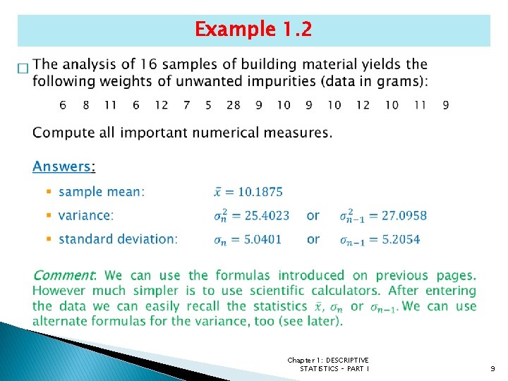
Example 1. 2 � Chapter 1: DESCRIPTIVE STATISTICS – PART I 9

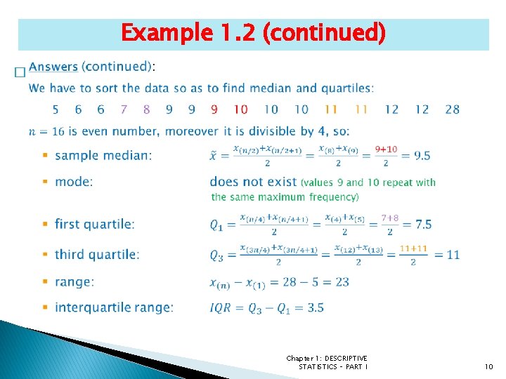
Example 1. 2 (continued) � Chapter 1: DESCRIPTIVE STATISTICS – PART I 10

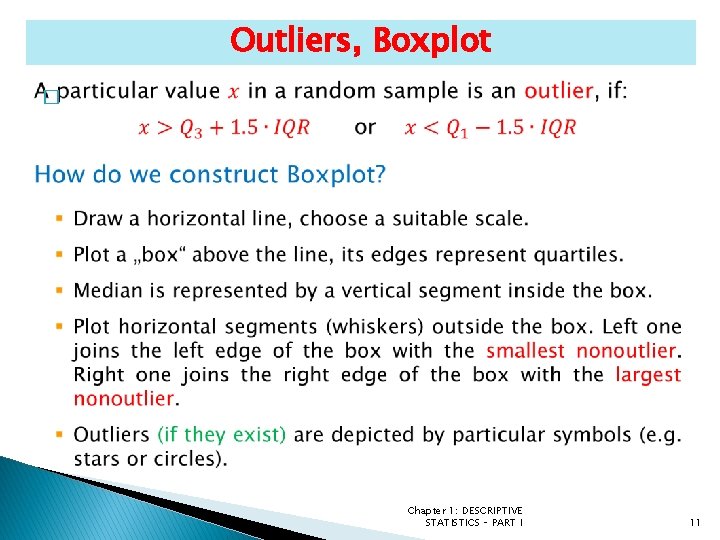
Outliers, Boxplot � Chapter 1: DESCRIPTIVE STATISTICS – PART I 11

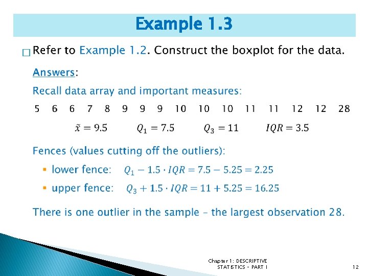
Example 1. 3 � Chapter 1: DESCRIPTIVE STATISTICS – PART I 12

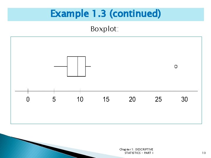
Example 1. 3 (continued) Boxplot: Chapter 1: DESCRIPTIVE STATISTICS – PART I 13

Example 1. 4 Refer to Examples 1. 2 and 1. 3: We found in Example 1. 3 that value 28 is an outlier. Assume that this value is an erroneous measurement and exclude it from the sample. a) Compute basic summary measures for the reduced sample of 15 observations. b) Construct the boxplot for the reduced sample. c) Compare the results for both samples. Answers are available on my personal website. Chapter 1: DESCRIPTIVE STATISTICS – PART I 14

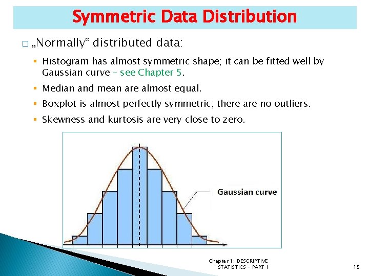
Symmetric Data Distribution � „Normally“ distributed data: § Histogram has almost symmetric shape; it can be fitted well by Gaussian curve – see Chapter 5. § Median and mean are almost equal. § Boxplot is almost perfectly symmetric; there are no outliers. § Skewness and kurtosis are very close to zero. Chapter 1: DESCRIPTIVE STATISTICS – PART I 15

Symmetric Data Distribution (continued) � Examples: § Histogram of compressive strength of concrete on page 4. § Boxplot constructed in Example 1. 4 (15 samples of building material – reduced data set). Comment: Skewness computed for the data in Example 1. 4 is negative and equals approx. -0. 416. It shows that there the data are actually gentle left skewed - see later. (You will not be asked to compute skewness in the exam. ) Chapter 1: DESCRIPTIVE STATISTICS – PART I 16

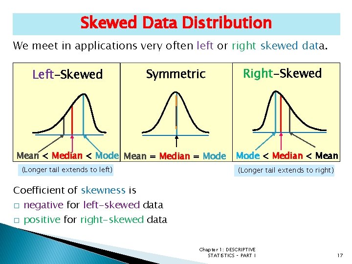
Skewed Data Distribution We meet in applications very often left or right skewed data. Left-Skewed Symmetric Mean < Median < Mode Mean = Median = Mode (Longer tail extends to left) Right-Skewed Mode < Median < Mean (Longer tail extends to right) Coefficient of skewness is � negative for left-skewed data � positive for right-skewed data Chapter 1: DESCRIPTIVE STATISTICS – PART I 17

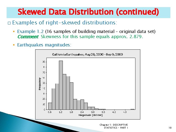
Skewed Data Distribution (continued) � Examples of right-skewed distributions: § Example 1. 2 (16 samples of building material – original data set) Comment: Skewness for this sample equals approx. 2. 879. § Earthquakes magnitudes: Chapter 1: DESCRIPTIVE STATISTICS – PART I 18

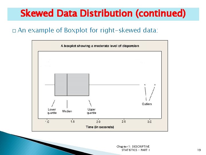
Skewed Data Distribution (continued) � An example of Boxplot for right-skewed data: Chapter 1: DESCRIPTIVE STATISTICS – PART I 19

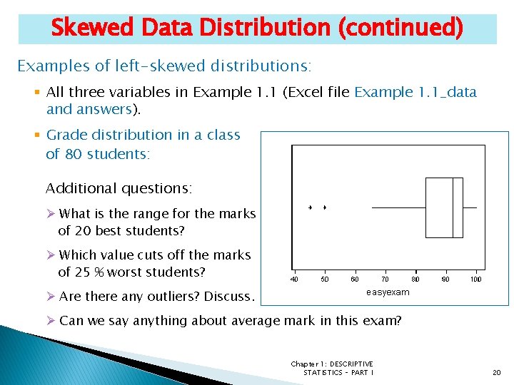
Skewed Data Distribution (continued) Examples of left-skewed distributions: § All three variables in Example 1. 1 (Excel file Example 1. 1_data and answers). § Grade distribution in a class of 80 students: Additional questions: Ø What is the range for the marks of 20 best students? Ø Which value cuts off the marks of 25 % worst students? Ø Are there any outliers? Discuss. Ø Can we say anything about average mark in this exam? Chapter 1: DESCRIPTIVE STATISTICS – PART I 20

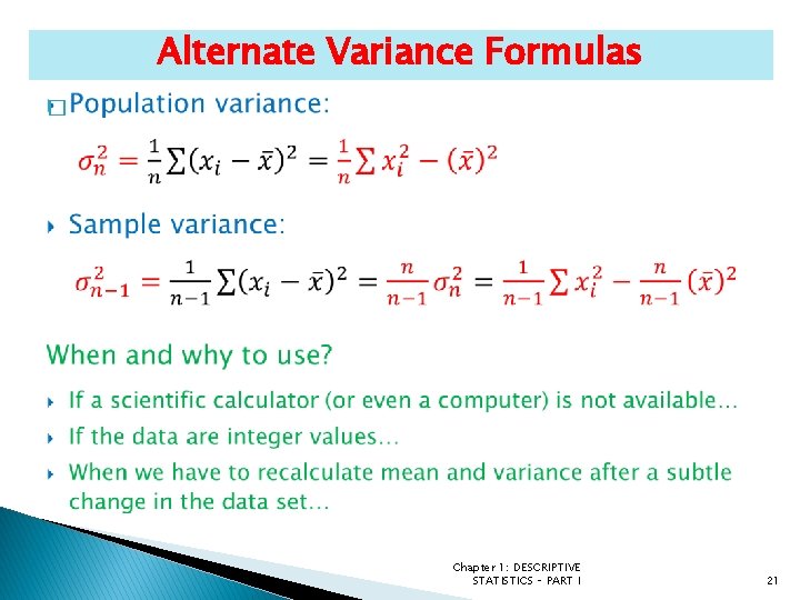
Alternate Variance Formulas � Chapter 1: DESCRIPTIVE STATISTICS – PART I 21

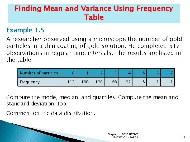
Finding Mean and Variance Using Frequency Table Example 1. 5 A researcher observed using a microscope the number of gold particles in a thin coating of gold solution. He completed 517 observations in regular time intervals. The results are listed in the table: Number of particles Frequency 0 1 2 3 4 5 6 7 112 168 130 68 32 5 1 1 Compute the mode, median, and quartiles. Compute the mean and standard deviation, too. Comment on the data distribution. Chapter 1: DESCRIPTIVE STATISTICS – PART I 22

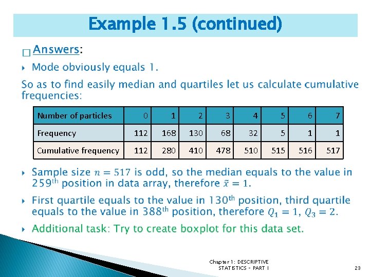
Example 1. 5 (continued) � Number of particles 0 1 2 3 4 5 6 7 Frequency 112 168 130 68 32 5 1 1 Cumulative frequency 112 280 410 478 510 515 516 517 Chapter 1: DESCRIPTIVE STATISTICS – PART I 23

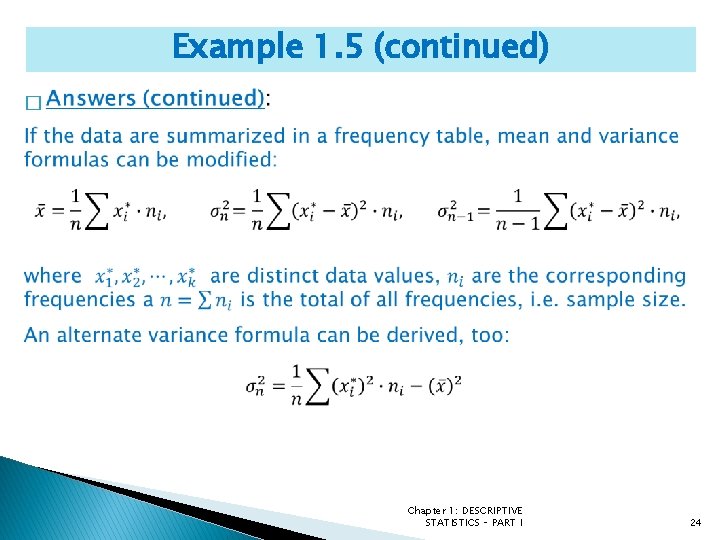
Example 1. 5 (continued) � Chapter 1: DESCRIPTIVE STATISTICS – PART I 24

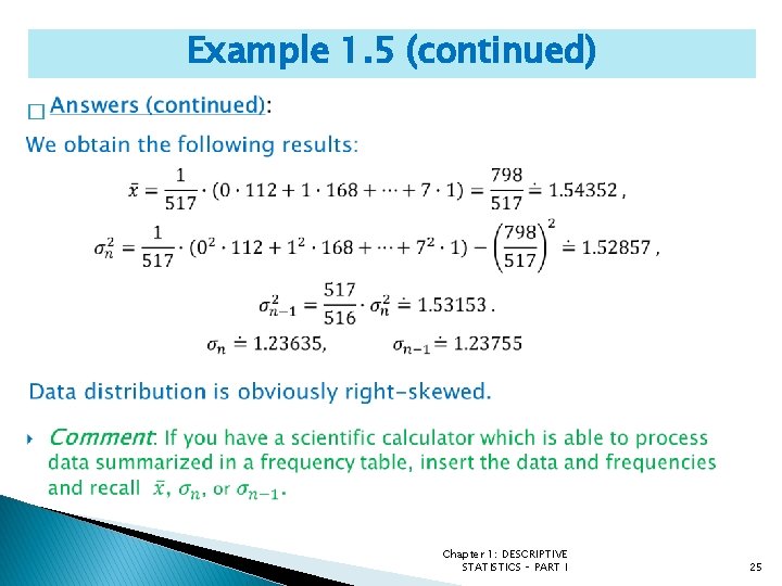
Example 1. 5 (continued) � Chapter 1: DESCRIPTIVE STATISTICS – PART I 25

Estimating Mean and Variance Using Grouped Frequency Table � Chapter 1: DESCRIPTIVE STATISTICS – PART I 26