Mathematical Statistics Lecture 13 Prof Dr M Junaid

Mathematical Statistics Lecture 13 Prof. Dr. M. Junaid Mughal 1

Last Class • • Introduction to Probability (continued) Random Variable Discrete and Continuous Random Variables Discrete Probability Distribution • Continuous Probability Distribution 2

Today’s Agenda • Review of – – – Discrete and Continuous Random Variables Discrete Probability Distribution Continuous Probability Distribution • Exercises 3

Random Variables • A random variable is a function that associates a real number with each element in the sample space. 4

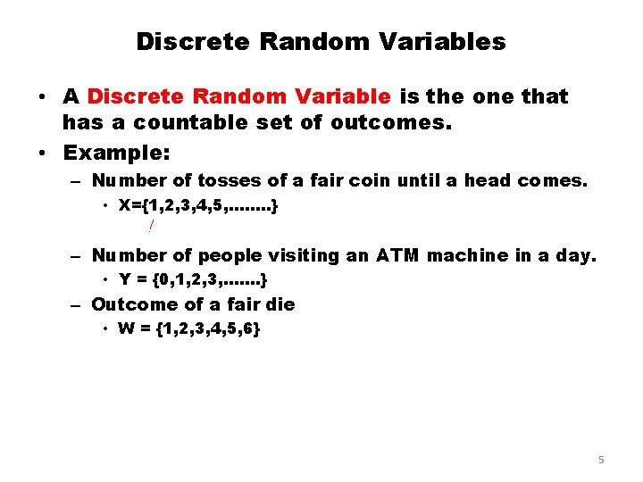
Discrete Random Variables • A Discrete Random Variable is the one that has a countable set of outcomes. • Example: – Number of tosses of a fair coin until a head comes. • X={1, 2, 3, 4, 5, ……. . } – Number of people visiting an ATM machine in a day. • Y = {0, 1, 2, 3, ……. } – Outcome of a fair die • W = {1, 2, 3, 4, 5, 6} 5

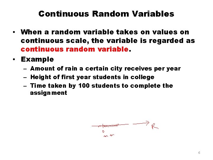
Continuous Random Variables • When a random variable takes on values on continuous scale, the variable is regarded as continuous random variable. • Example – Amount of rain a certain city receives per year – Height of first year students in college – Time taken by 100 students to complete the assignment 6

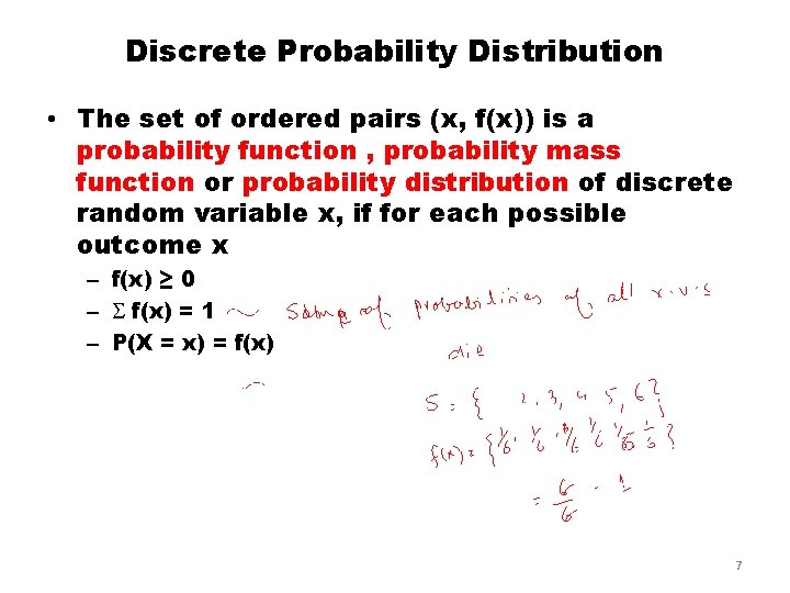
Discrete Probability Distribution • The set of ordered pairs (x, f(x)) is a probability function , probability mass function or probability distribution of discrete random variable x, if for each possible outcome x – f(x) ≥ 0 – f(x) = 1 – P(X = x) = f(x) 7

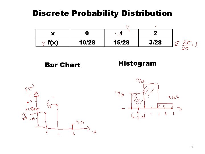
Discrete Probability Distribution x 0 1 2 f(x) 10/28 15/28 3/28 Bar Chart Histogram 8

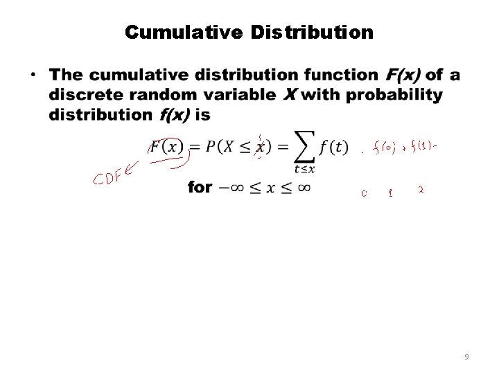
Cumulative Distribution • 9

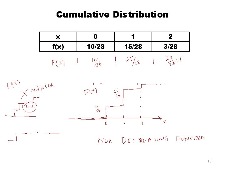
Cumulative Distribution x 0 1 2 f(x) 10/28 15/28 3/28 10

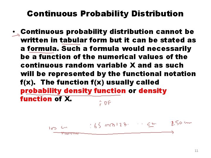
Continuous Probability Distribution • Continuous probability distribution cannot be written in tabular form but it can be stated as a formula. Such a formula would necessarily be a function of the numerical values of the continuous random variable X and as such will be represented by the functional notation f(x). The function f(x) usually called probability density function or density function of X. 11

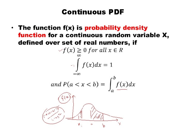
Continuous PDF •

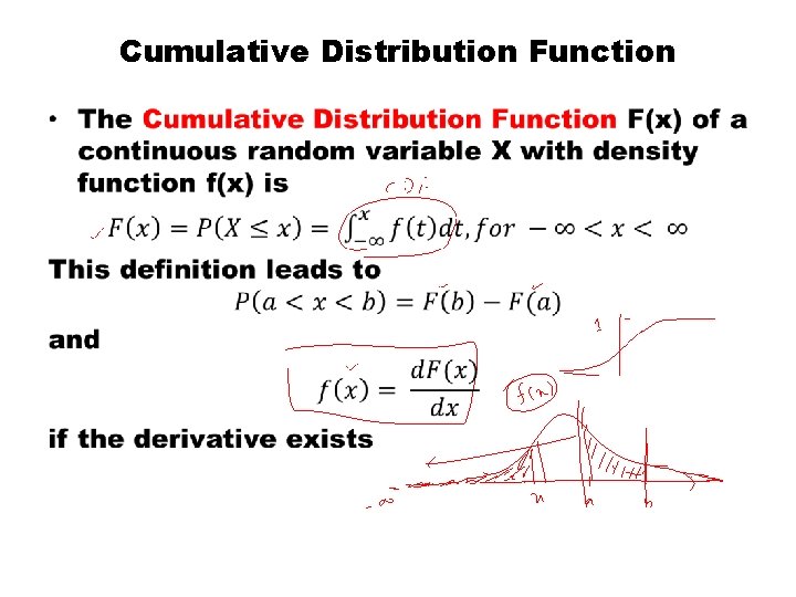
Cumulative Distribution Function •

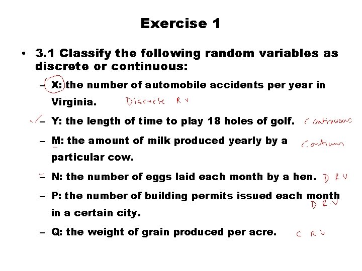
Exercise 1 • 3. 1 Classify the following random variables as discrete or continuous: – X: the number of automobile accidents per year in Virginia. – Y: the length of time to play 18 holes of golf. – M: the amount of milk produced yearly by a particular cow. – N: the number of eggs laid each month by a hen. – P: the number of building permits issued each month in a certain city. – Q: the weight of grain produced per acre.

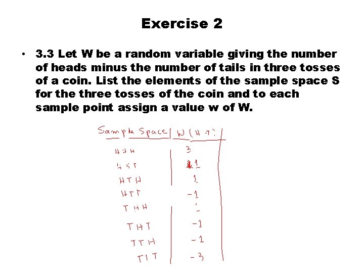
Exercise 2 • 3. 3 Let W be a random variable giving the number of heads minus the number of tails in three tosses of a coin. List the elements of the sample space S for the three tosses of the coin and to each sample point assign a value w of W.

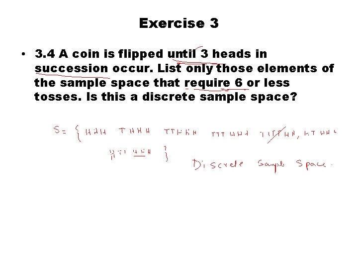
Exercise 3 • 3. 4 A coin is flipped until 3 heads in succession occur. List only those elements of the sample space that require 6 or less tosses. Is this a discrete sample space?

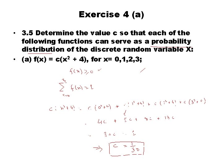
Exercise 4 (a) • 3. 5 Determine the value c so that each of the following functions can serve as a probability distribution of the discrete random variable X: • (a) f(x) = c(x 2 + 4), for x= 0, 1, 2, 3;

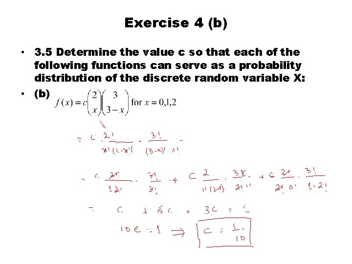
Exercise 4 (b) • 3. 5 Determine the value c so that each of the following functions can serve as a probability distribution of the discrete random variable X: • (b)

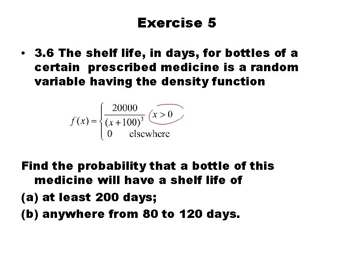
Exercise 5 • 3. 6 The shelf life, in days, for bottles of a certain prescribed medicine is a random variable having the density function Find the probability that a bottle of this medicine will have a shelf life of (a) at least 200 days; (b) anywhere from 80 to 120 days.

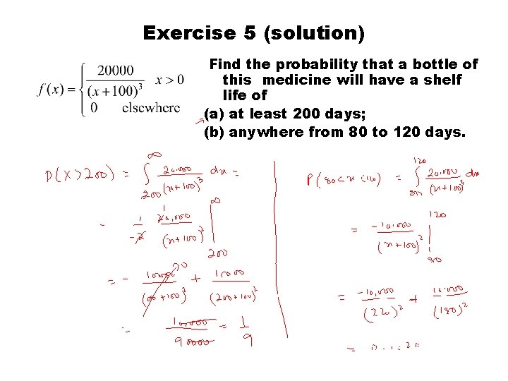
Exercise 5 (solution) Find the probability that a bottle of this medicine will have a shelf life of (a) at least 200 days; (b) anywhere from 80 to 120 days.

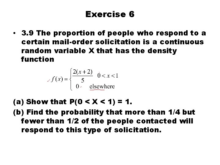
Exercise 6 • 3. 9 The proportion of people who respond to a certain mail-order solicitation is a continuous random variable X that has the density function (a) Show that P(0 < X < 1) = 1. (b) Find the probability that more than 1/4 but fewer than 1/2 of the people contacted will respond to this type of solicitation.

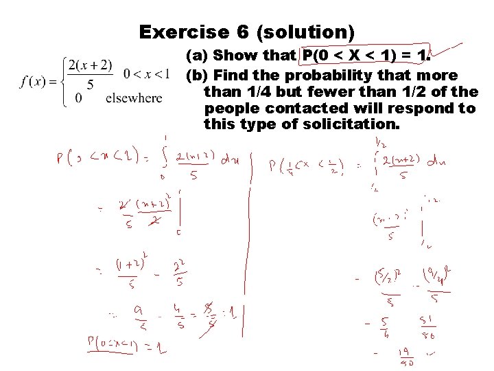
Exercise 6 (solution) (a) Show that P(0 < X < 1) = 1. (b) Find the probability that more than 1/4 but fewer than 1/2 of the people contacted will respond to this type of solicitation.

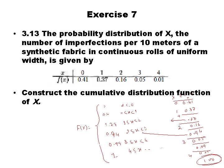
Exercise 7 • 3. 13 The probability distribution of X, the number of imperfections per 10 meters of a synthetic fabric in continuous rolls of uniform width, is given by • Construct the cumulative distribution function of X.

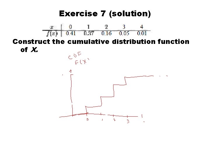
Exercise 7 (solution) Construct the cumulative distribution function of X.

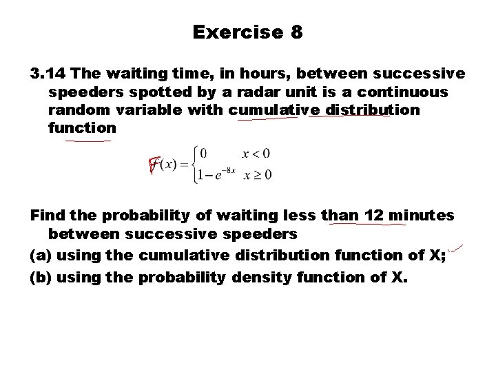
Exercise 8 3. 14 The waiting time, in hours, between successive speeders spotted by a radar unit is a continuous random variable with cumulative distribution function Find the probability of waiting less than 12 minutes between successive speeders (a) using the cumulative distribution function of X; (b) using the probability density function of X.

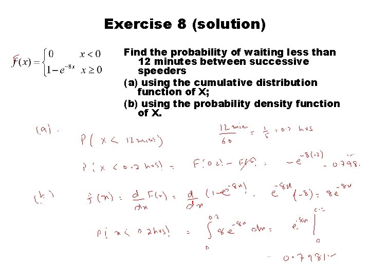
Exercise 8 (solution) Find the probability of waiting less than 12 minutes between successive speeders (a) using the cumulative distribution function of X; (b) using the probability density function of X.

Summary • Random Variable • Probability Distributions References • Probability and Statistics for Engineers and Scientists by Walpole • Schaum outline series in Probability and Statistics 27

Example