Mathematical Models of Physical Systems Why mathematical models

Mathematical Models of Physical Systems • Why mathematical models of physical systems needed? • Design of engineering systems by trying and error versus design by using mathematical models. • Physical laws such as Newton’s second law of motion is a mathematical model. • Mathematical model gives the mathematical relationships relating the output of a system to its input.

Mathematical Models of Physical Systems (continued) • Control systems give desired output by controlling the input. Therefore control systems and mathematical modeling are inter-linked. • Mathematical models of control systems are ordinary differential equations • To deal with linear o. d. e, Laplace Transform is an efficient approach.

What is Laplace Transform? • The Laplace transform of a function f(t) is defined as: • The inverse Laplace transform is defined as: where and the value of is determined by the singularities of F(s).

Why Is Laplace Transform Useful ? • Model a linear time-invariant analog system as an algebraic system (transfer function). • In control theory, Laplace transform converts linear differential equations into algebraic equations. • This is much easier to manipulate and analyze.

An Example • The Laplace transform of can be obtained by: Linearity property • These are useful properties:

Name Unit Impulse Unit Step Unit ramp nth-Order ramp Exponential Time function f(t) u(t) t tn e-at nth-Order exponential t n e-at Sine sin(bt) Cosine cos(bt) Damped sine e-at sin(bt) Damped cosine e-at cos(bt) Diverging sine t sin(bt) Diverging cosine t cos(bt) Laplace Transform 1 1/s 2 n!/sn+1 1/(s+a) n!/(s+a)n+1 b/(s 2+b 2) s/(s 2+b 2) b/((s+a)2+b 2) (s+a)/((s+a)2+b 2) 2 bs/(s 2+b 2)2 (s 2 -b 2) /(s 2+b 2)2

table_02_02

Find the Laplace transform of f(t)=5 u(t)+3 e -2 t. • Solution:

Partial Fraction Expansion (Case 1: Roots of Denominator are Real and distinct) Find the inverse Laplace transform of F(s)=5/(s 2+3 s+2). Solution:

Exercise: Do example 2. 3 of the textbook Laplace Transform solution of a differential equation

Case 2: Roots of the Denominator are Real and Repeated

Case 2: continue of the example F(s)=(2 s+3)/(s 3+2 s 2+s).

Case 3: Roots of the Denominator are Complex. Example: F(s)=10/(s 3+4 s 2+9 s+10)

For the Tutorial next week, use Matlab to find the Inverse Laplace Transform for the case where the roots of the denominator are complex roots.

The Transfer Function

Transfer Function for a differential equation Exercise: Do examples 2. 4 and 2. 5 on the Textbook.

Models of Electrical Circuits • Resistance circuit: v(t) = i(t) R • Inductance circuit: •

Models of Electrical Circuits • Capacitance circuit:

Transfer Functions for Electrical Networks

• Kirchhoff’ s voltage law: The algebraic sum of voltages around any closed loop in an electrical circuit is zero. • Kirchhoff’ s current law: The algebraic sum of currents into any junction in an electrical circuit is zero.

Electrical network (Example 2. 6) Original network Transfer Function network Laplace Transform network

• Exercise: Do example 2. 10 of the textbook • Excluding Operational Amplifiers

fig_02_06

Models of Mechanical Systems Mechanical translational systems. • Newton’s second law: • Device with friction (shock absorber): B is damping coefficient. • Translational system to be defined is a spring (Hooke’s law): K is spring coefficient

table_02_04

• Model of a mass-spring-damper system: • Note that linear physical systems are modeled by linear differential equations for which linear components can be added together. See example of a mass-spring-damper system.

Transfer Functions for Mechanical Systems

Exercise: Do example 2. 17 of the text

fig_02_17

fig_02_18

fig_02_19

Mechanical Rotational Systems • Moment of inertia: • Viscous friction: • Torsion:

table_02_05

• Model of a torsional pendulum (pendulum in clocks inside glass dome): Moment of inertia of pendulum bob denoted by J Friction between the bob and air by B Elastance of the brass suspension strip by K

Transfer Functions for Systems with Gears

fig_02_29

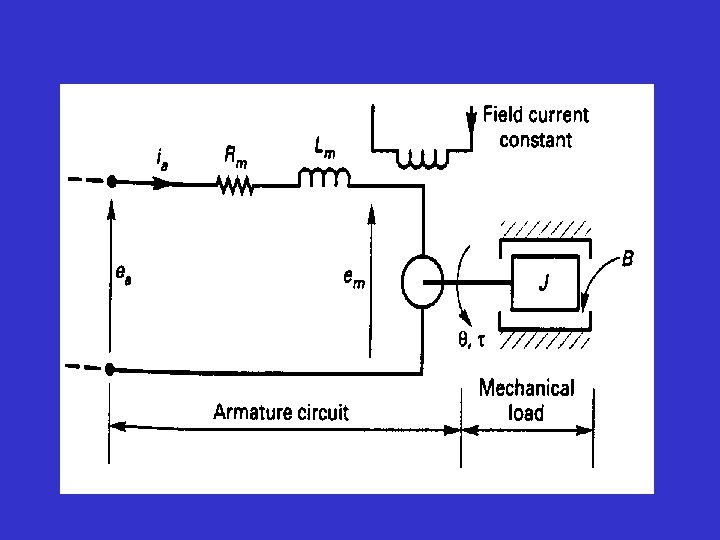
Electro-mechanical System Transfer Functions

Equivalence between Mechanical and Electrical Systems

• Differential equations as mathematical models of physical systems: similarity between mathematical models of electrical circuits and models of simple mechanical systems (see model of an RCL circuit and model of the mass-spring-damper system).

This leads to the concept of the Transfer Function which is the corner stone of the control theory. Transfer functions are defined from the Laplace Transform.

• Summary of through- and across-variables for physical systems: System Variable Through Element Integrated Through Variable Across Integrated Element Across Variable Electrical Current, i Charge, q Voltage difference, 21 Flux linkage, 21 Mechanical Force, F Translational momentum, P Velocity difference, 21 Displacement difference, y 21 Mechanical rotational Torque, T Angular momentum, h Angular velocity difference, 21 Angular displacement difference, 21 Fluid volumetric rate of flow, Q Volume, V Pressure difference, P 21 Pressure momentum, 21 Thermal Heat flow rate, q Heat energy, Temperature difference, 21 H

• Model of electromechanical systems. • Model of a servomotor:

• Model of temperature-control system: heat flow given by electric heater heat flow via liquid entering tank heat flow into liquid heat flow via liquid leaving tank heat flow (loss) via tank surface H = specific heat of liquid C = thermal capacity R = thermal resistance V = volume of liquid