Mathematical Models of Climate Change The good the

Mathematical Models of Climate Change: The good, the bad and the ugly Chris Budd

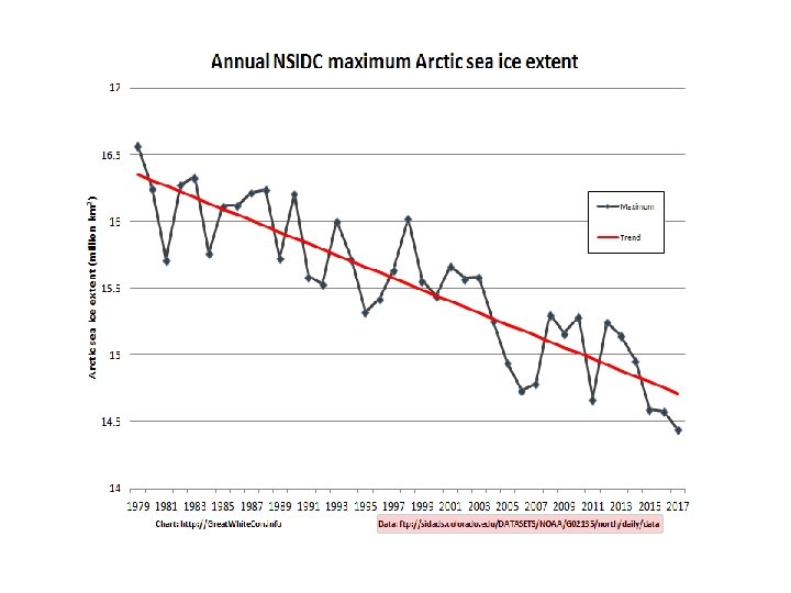
Our climate is changing! Both now (rapidly)

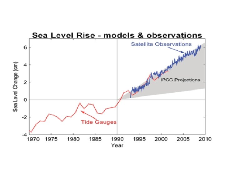
Sea level rise

And in the past (more slowly)

The IPCC relies on (mathematical) models to both help predict the future climate to understand past climate

Models make predictions and come with a level of uncertainty

Modern Global Climate Models GCMs are highly complex with billions of degrees of freedom and take large parallel computers to run Moss et. Al. , (2010) Nature

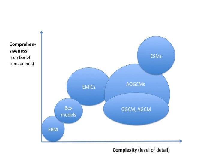
All models are based on mathematics, coupled with physics, chemistry, biology, astrophysics, . . GCM: Global models of climate change. Complex with millions of lines of code. Look at whole Earth, oceans and atmosphere. Effective for precise predictions over decades. EMIC: Less complex intermediate models of the physics. Treat Earth as a series of boxes. Make predictions over much longer periods. Useful to test models, verify GCM predictions, predict ice ages EBM: Simplest models. Treat Earth as a single point. Look at balances of energy, albedo and other effects. Good for sensitivity calculations

Met Office hierarchy of weather and climate models UK Hadley Centre

Modelling the climate accurately is hard It is difficult to predict anything, especially about the future! Niels Bohr Some reasons for the uncertainty Statistical variations in hard to measure data Chaos and nonlinearity Complexity of the system Distinguishing between cause and effect eg. Temp and CO 2 Distinguishing between natural and human made variation

Leads to uncertainty, concern and misunderstanding

Climate has always been changing All climate change is due to the Sun Quotes from the comments section on my videos Problem with the temperature chart. It's showing it warmer than the 1930 s when the US had record highs close to 100 nationwide. The big problem is that they assume that rising CO 2 level result in rising temperature, correlation is not causation. The ice core samples show an 800 year lag temperatures rise, plants grow, oceans warm releasing more CO 2. Temperatures drop, vegetation recedes, oceans cool, CO 2 follows after the temp. CO 2 is therefore not the cause of warming, but the effect CO 2 does not harm the planet. You don't need a degree in math to understand that. Maths? Climate change is not maths! It is Physics. Or don't you agree?

Despite/because of all of this …. Mathematics/statistical modelling is still our best tool for • Being objective in our analysis and understanding of climate change • Understanding sensitivity and time scales and the reasons for extreme events • Understanding the relation between causes and effects over both long and short terms • Predicting the effects of climate change eg. Flooding, food

The modelling process All climate models start with the laws of physics Are formulated as (partial) differential equations Incorporate data Quantify uncertainty Are solved numerically

What makes up the climate? Air Pressure p Air Velocity u Air/Ocean Temperature T Air density Moisture/clouds q Same for the oceans + ice + salt All affected by: Solar radiation S(t) Earth’s rotation f Gravity g Mountains, vegetation, ice, CO 2, Human activity

Complex interrelated processes described by differential equations Basic equations: Navier-Stokes which describe the weather Motion Density Temperature Moisture Pressure For climate add in ice, CO 2, ocean currents, vegetation, …

[Hadley Centre]

Discretise the PDEs and solve on a (super) computer 100 km

Test GCMs by hind casting on past data (c) Natural and anthropogenic IPCC

Future predictions Hansen et. al. (1981), Science Prediction made using an energy balance model with a climate sensitivity of 2. 8 C per doubling of CO 2

Examples of simpler models Energy Balance Model (EBM) [Arrhenius]

Total Incoming solar radiation S(t) (short wave radiation) Amount absorbed (1 – a) S(t)/4 Space Atmosphere Earth Energy flux from atmosphere

Energy is received by Earth as short wave radiation Reradiated from the Earth as long wave radiation Energy absorbed and reradiated from the atmosphere Flux balance 1:

Flux balance 2: Short wave transparency 0. 9 Long wave transparency 0. 2

Power of this model is its ability to make predictions of the sensitivity of the Earth to changes in CO 2 and e decrease with CO 2 content increases

However, albedo is directly linked to temperature This significantly increases the sensitivity of the temperature to changes in Carbon Dioxide

Can also ‘predict’ Tipping Points Hot Earth Cold ‘Snowball’ Earth

But the model is BAD for doing this as it takes no account of the time-scales of the: • Radiation • Ice melting • Ocean Currents • CO 2 feedback Can use BETTER EMIC models to study climate eg. ice ages looking more at the coupling between ice, temperature and CO 2 and including time-scales

Such models need to be able to explain the periodicity of the ice ages AND the Mid-Pleistocene Transition (MPT) 41 kyr cycle 100 kyr cycle

Variety of low-dimensional dynamical systems models are used to model this Classical dynamical systems: Smooth evolution. Hopf bifurcations for the transitions Non-smooth dynamical systems and relaxation oscillators Switches and very different time-scales for the evolution. Grazing bifurcations for the transitions.

Key factor: S(t) varies due to Milankovich cycles S(t) = I_65

Issues: 1. 19 kyr, 23 kr, 41 kyr cycles all significant implying linear forcing before the MPT 2. 100 kr eccentricity variation: very small forcing!! Q. Is the recent 100 kyr cycle A. Forced by the eccentricity changes B. Weakly synchronised by the eccentricity changes C. Independent of these changes and instead caused by an internal climate variation which also has a 100 kyr period eg. Ice sheet growth

[Saltzman + Maasch 1990, 1991] V: Ice mass T: Deep ocean temperature C: CO 2 Parameters CHOSEN to give 100 kyr cycle Carbon Cycle model CO 2 Tectonic plate forcing

Predicts: Hopf bifurcation as an explanation for the MPT Bifurcation occurs due to a slow variation in CO 2 forcing Linear Nonlinear regime before MPT regime after MPT (forced) (synchronised) But …. Crucial CO 2 equation very contrived! No real justification!

Relaxation Oscillator Models [Paillard], [Ashwin], [review in Crucifix] [B and Morupisi] These model the climate as a multi-equilibrium system which relaxes to a set of different states. Transitions between the states are generated using nonsmooth maps which can be modelled using hybrid dynamical systems or by using a slow manifold Can give some explanation for the MPT transition

Paillard and Parrenin (2004) V: Ice volume A: Antarctic Ice Model: atmospheric Carbon Dioxide rapidly increases when Southern Ocean suddenly ventilates Ventilation occurs when deep ocean stratification ceases Release of Carbon Dioxide leads to warming of the Earth which drives a rapid deglaciation process PP 04 Transition Model C: Carbon Dioxide

Heavyside function V: Ice volume A: Antarctic Ice C: Carbon Dioxide Stratification parameter or Salt water formation efficiency

C A V I_65 F

(1, 2) periodic orbit (1, 3) periodic orbit Co-existence of periodic states

(1, 2) periodic orbit (1, 3) periodic orbit

Domain of attraction (1, 3) orbit (1, 2) Grazing line (1, 3) orbit

Graze Transition similar to the MPT

PP 04 model with quasiperiodic forcing Observations

Conclusions • Mathematical models are the best way to predict future climate and to understand past climate • A hierarchy of models is needed to make useful predictions over a full range of time and length scales • Models are only as good as the physics and data underlying them • But do this correctly and you should get the right answer