Mathematical Foundations of AI Lecture 2 CSP Tractability
Mathematical Foundations of AI Lecture 2 - CSP Tractability due to restricted structure Reshef Meir, Hebrew University, 2011
Lecture content • Constraint Satisfaction Problems • CSP on trees • Hyper-trees and join-trees • Tree decomposition
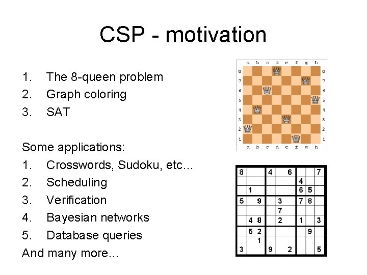
CSP - motivation 1. 2. 3. The 8 -queen problem Graph coloring SAT Some applications: 1. Crosswords, Sudoku, etc… 2. Scheduling 3. Verification 4. Bayesian networks 5. Database queries And many more…
Constraint Satisfaction Problems • Definition: A constraint satisfaction problem is defined as a triple (X, d, C) – X is a set of variables in the range {1, 2, …, d} • The range is known as the domain of the variable – C is a set of constraints C 1(S 1). . . Cn(Sn) where each Si X is a set of variables. A solution to the CSP is an assignment of values to x 1…xn that satisfies all constraints.
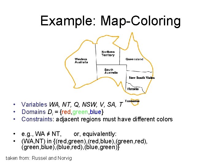
Example: Map-Coloring • Variables WA, NT, Q, NSW, V, SA, T • Domains Di = {red, green, blue} • Constraints: adjacent regions must have different colors • e. g. , WA ≠ NT, or, equivalently: • (WA, NT) in {(red, green), (red, blue), (green, red), (green, blue), (blue, red), (blue, green)} taken from: Russel and Norvig
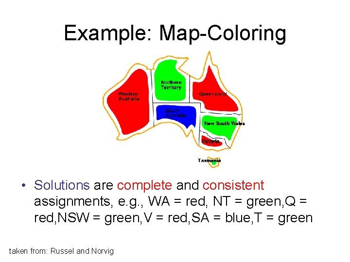
Example: Map-Coloring • Solutions are complete and consistent assignments, e. g. , WA = red, NT = green, Q = red, NSW = green, V = red, SA = blue, T = green taken from: Russel and Norvig
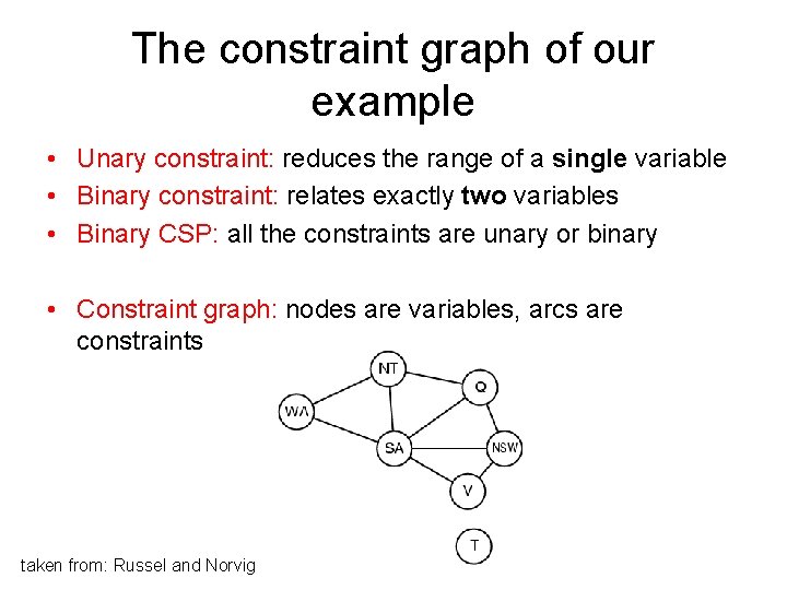
The constraint graph of our example • Unary constraint: reduces the range of a single variable • Binary constraint: relates exactly two variables • Binary CSP: all the constraints are unary or binary • Constraint graph: nodes are variables, arcs are constraints taken from: Russel and Norvig
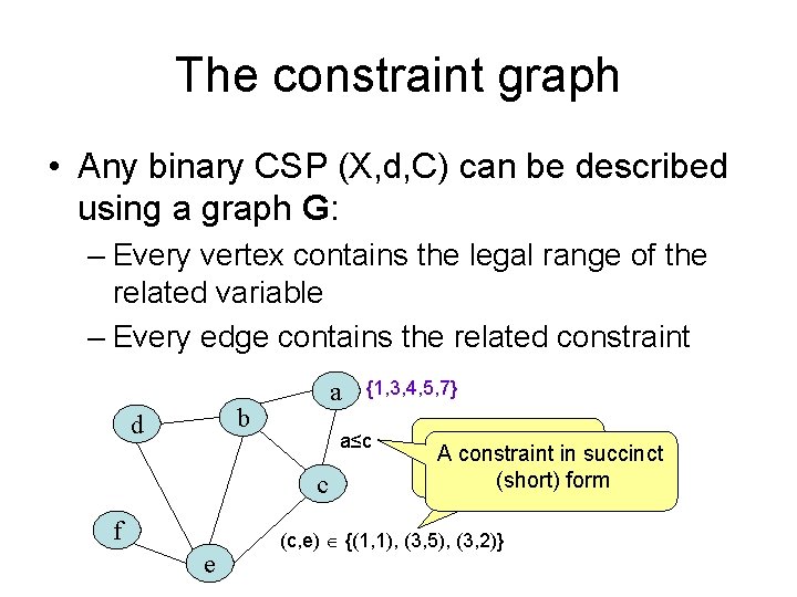
The constraint graph • Any binary CSP (X, d, C) can be described using a graph G: – Every vertex contains the legal range of the related variable – Every edge contains the related constraint a b d a≤c c f e {1, 3, 4, 5, 7} A constraint in succinct in full form (short) form (c, e) {(1, 1), (3, 5), (3, 2)}
Try 1: Backtracking search • Consider a tree of depth n, containing all assignments of x 1, x 2, …, xn • Need to consider a single variable at each node branching factor = d there are dn leaves • Depth-first search for CSPs with single-variable assignments is called backtracking search • Can solve n-queens for n ≈ 25
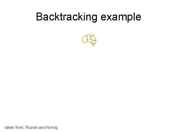
Backtracking example taken from: Russel and Norvig
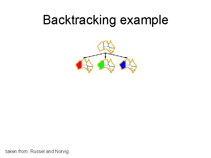
Backtracking example taken from: Russel and Norvig
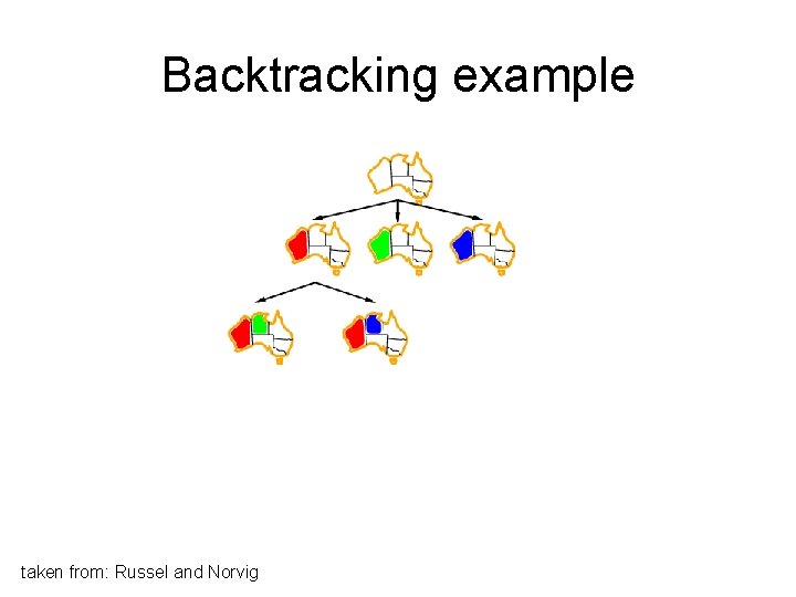
Backtracking example taken from: Russel and Norvig
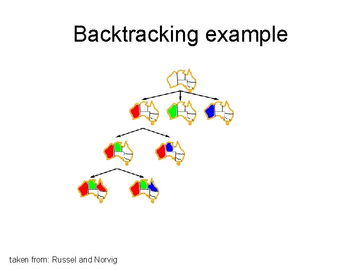
Backtracking example taken from: Russel and Norvig
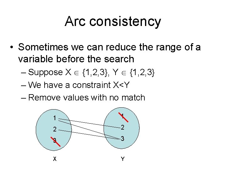
Arc consistency • Sometimes we can reduce the range of a variable before the search – Suppose X {1, 2, 3}, Y {1, 2, 3} – We have a constraint X<Y – Remove values with no match 1 1 2 2 3 3 X Y
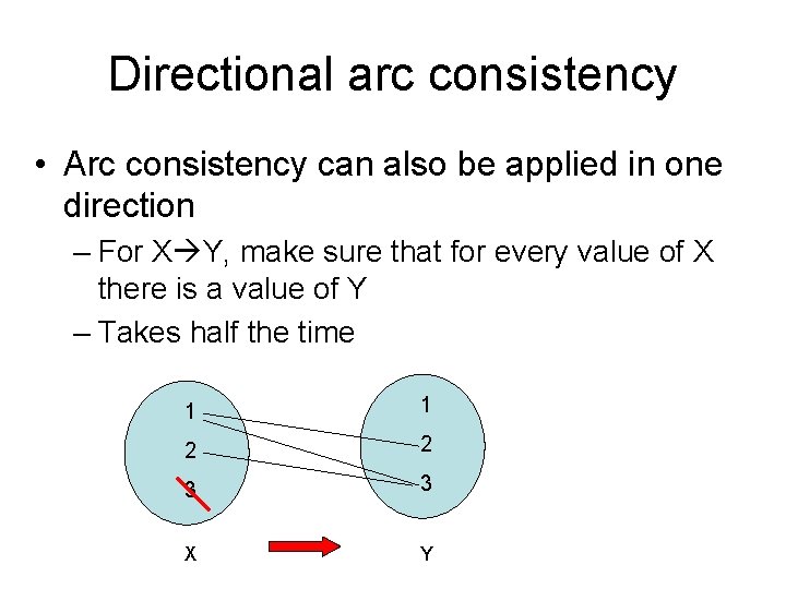
Directional arc consistency • Arc consistency can also be applied in one direction – For X Y, make sure that for every value of X there is a value of Y – Takes half the time 1 1 2 2 3 3 X Y
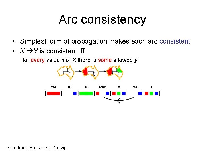
Arc consistency • Simplest form of propagation makes each arc consistent • X Y is consistent iff for every value x of X there is some allowed y taken from: Russel and Norvig

Arc consistency • Simplest form of propagation makes each arc consistent • X Y is consistent iff for every value x of X there is some allowed y taken from: Russel and Norvig
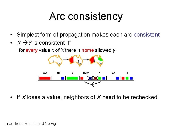
Arc consistency • Simplest form of propagation makes each arc consistent • X Y is consistent iff for every value x of X there is some allowed y • If X loses a value, neighbors of X need to be rechecked taken from: Russel and Norvig
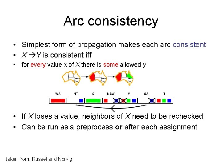
Arc consistency • Simplest form of propagation makes each arc consistent • X Y is consistent iff • for every value x of X there is some allowed y • If X loses a value, neighbors of X need to be rechecked • Can be run as a preprocess or after each assignment taken from: Russel and Norvig
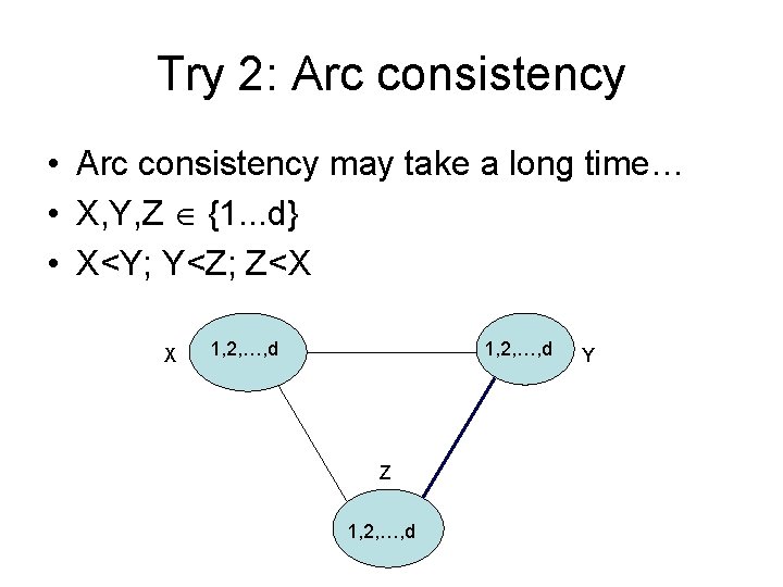
Try 2: Arc consistency • Arc consistency may take a long time… • X, Y, Z {1. . . d} • X<Y; Y<Z; Z<X X 1, 2, …, d Z 1, 2, …, d Y
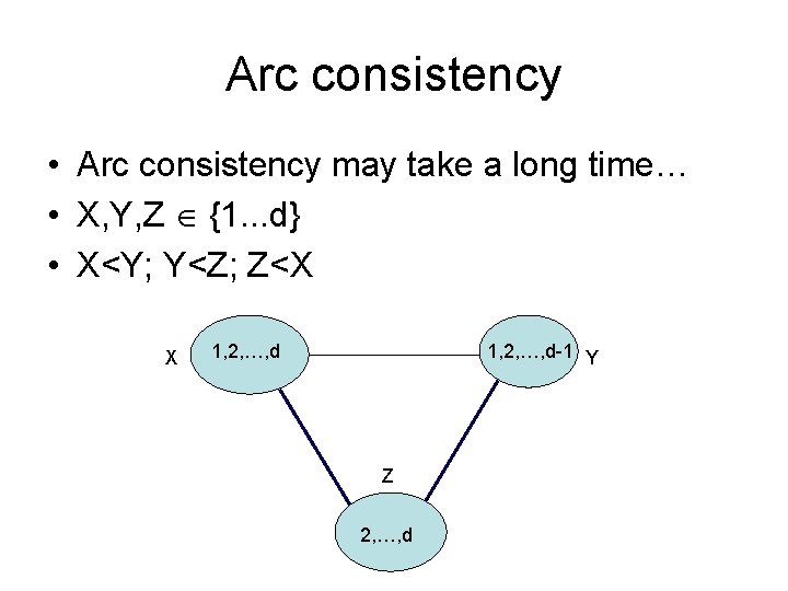
Arc consistency • Arc consistency may take a long time… • X, Y, Z {1. . . d} • X<Y; Y<Z; Z<X X 1, 2, …, d-1 Y Z 2, …, d
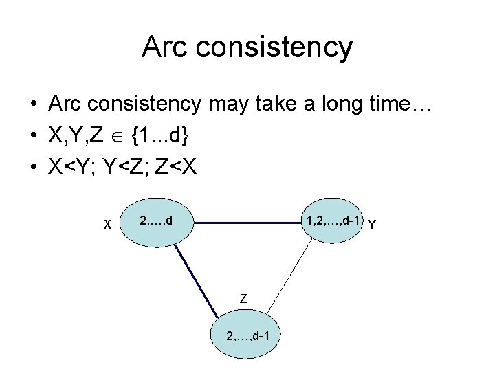
Arc consistency • Arc consistency may take a long time… • X, Y, Z {1. . . d} • X<Y; Y<Z; Z<X X 2, …, d 1, 2, …, d-1 Y Z 2, …, d-1
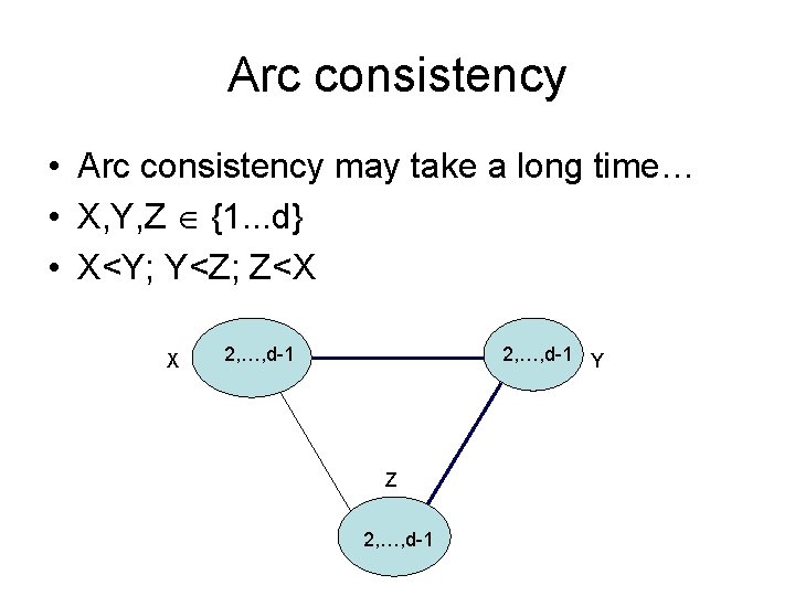
Arc consistency • Arc consistency may take a long time… • X, Y, Z {1. . . d} • X<Y; Y<Z; Z<X X 2, …, d-1 Y Z 2, …, d-1
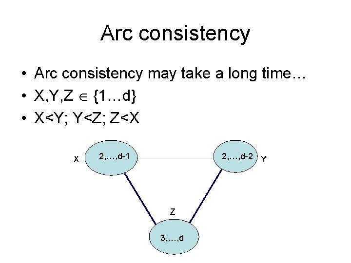
Arc consistency • Arc consistency may take a long time… • X, Y, Z {1…d} • X<Y; Y<Z; Z<X X 2, …, d-1 2, …, d-2 Y Z 3, …, d
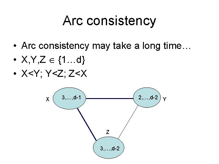
Arc consistency • Arc consistency may take a long time… • X, Y, Z {1…d} • X<Y; Y<Z; Z<X X 3, …, d-1 2, …, d-2 Y Z 3, …, d-2
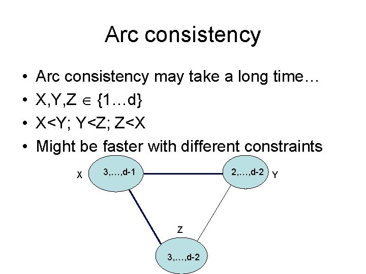
Arc consistency • • Arc consistency may take a long time… X, Y, Z {1…d} X<Y; Y<Z; Z<X Might be faster with different constraints X 3, …, d-1 2, …, d-2 Y Z 3, …, d-2
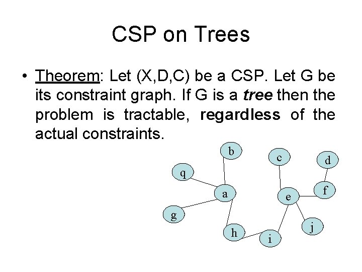
CSP on Trees • Theorem: Let (X, D, C) be a CSP. Let G be its constraint graph. If G is a tree then the problem is tractable, regardless of the actual constraints. b c d q a f e g h i j
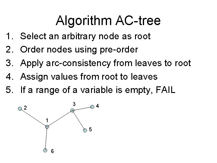
Algorithm AC-tree 1. 2. 3. 4. 5. Select an arbitrary node as root Order nodes using pre-order Apply arc-consistency from leaves to root Assign values from root to leaves If a range of a variable is empty, FAIL 3 2 4 1 1 5 6 2 3 4 5 6
Arc consistency and trees • Claim: algorithm AC-tree finds a legal value if there is one, and fails otherwise. • Runtime: O(n*d 2)
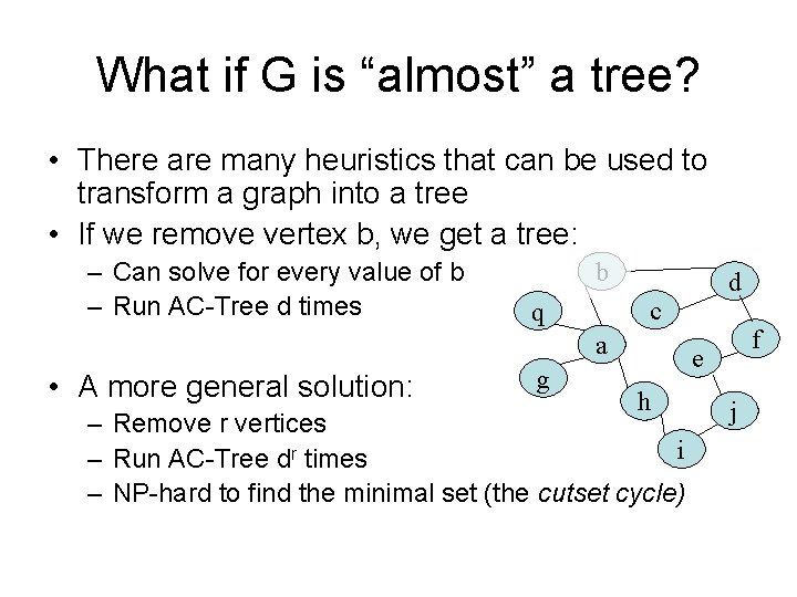
What if G is “almost” a tree? • There are many heuristics that can be used to transform a graph into a tree • If we remove vertex b, we get a tree: – Can solve for every value of b – Run AC-Tree d times b c q a • A more general solution: g d f e h – Remove r vertices i – Run AC-Tree dr times – NP-hard to find the minimal set (the cutset cycle) j
Non-binary constraint graphs • In the general case, a constraint may apply to more than two variables – E. g. 1: A+B=C – E. g. 2: A, B, C cannot have the same value • This results in a hyper-graph, instead of a a graph – An “edge” in a hyper graph is a set of vertices • Is there an equivalent concept for a “tree”?
Primal and dual graphs • Every hyper graph H induces two important graphs: the primal and the dual • Properties of these graphs can tell us valuable information on H. • The primal graph π(H): – Same vertices as in H – Connect a pair of vertices, if they share a constraint in H – H, H’ may have the same primal graph
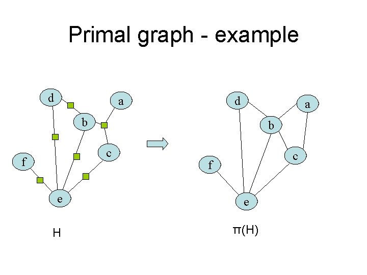
Primal graph - example d d a a b b c f e e H π(H)
The dual graph • The dual graph of H is a binary constraint graph • D(H) contains a vertex for every constraint in H – The range of the vertex v=(x 1, x 2, …xr) contains all the legal values of the r-tuple in H. • D(H) has an edge (binary constraint) between every pair of vertices that contain the same variable – The edge constrain the two copies of the variable to have the same value • D(H) is an injective ( if H≠H’ then D(H)≠D(H’) )
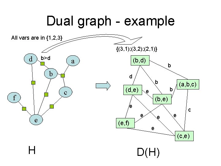
Dual graph - example All vars are in {1, 2, 3} {(3, 1); (3, 2); (2, 1)} d b>d a (b, d) b d c f b b (d, e) (a, b, c) b e (b, e) e e e (e, f) e e c e (c, e) H D(H)
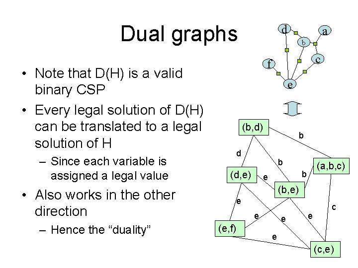
Dual graphs b c e (b, d) b d b (d, e) (a, b, c) b e (b, e) • Also works in the other direction – Hence the “duality” a f • Note that D(H) is a valid binary CSP • Every legal solution of D(H) can be translated to a legal solution of H – Since each variable is assigned a legal value d e e (e, f) e e c e (c, e)
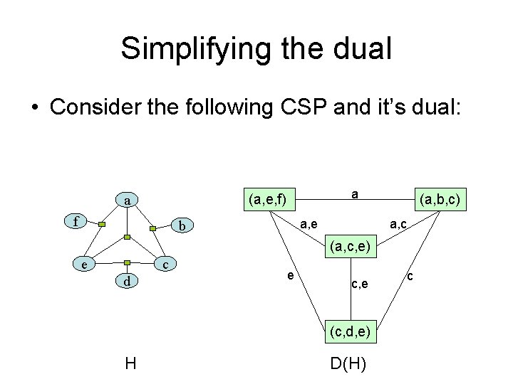
Simplifying the dual • Consider the following CSP and it’s dual: a (a, e, f) a f a, e b (a, b, c) a, c (a, c, e) c e d e c, e (c, d, e) H D(H) c

Simplifying the dual • Some edges in the dual can be safely removed • In fact, in this case we are left with a tree! • This is called the join tree H, or JT(H) a (a, e, f) a f a, e b (a, b, c) a, c (a, c, e) c e d e c, e (c, d, e) H D(H) c
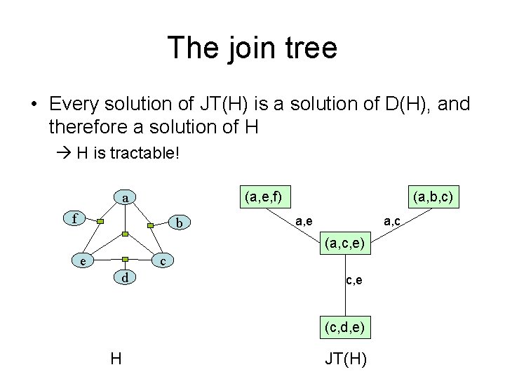
The join tree • Every solution of JT(H) is a solution of D(H), and therefore a solution of H H is tractable! (a, e, f) a f b (a, b, c) a, e a, c (a, c, e) c e d c, e (c, d, e) H JT(H)
Hyper trees • If a CSP H has a join tree, it is called uncyclic (sometimes also a hyper-tree). – There may be more than one join tree • Problem I: Most hyper-trees are cyclic, i. e. they have no join trees • Problem II: even if there is a join tree for H, it might be hard to find it – Edges might be removed in a wrong order – Exercise: show an example
Join tree verification • • Suppose we guess, or given, a subgraph T of the dual D(H) How can we tell if T is a valid join tree of H? 1. T is a tree 2. For every variable xi, there is a path in T between every two vertices containing xi, where xi appears in every edge.
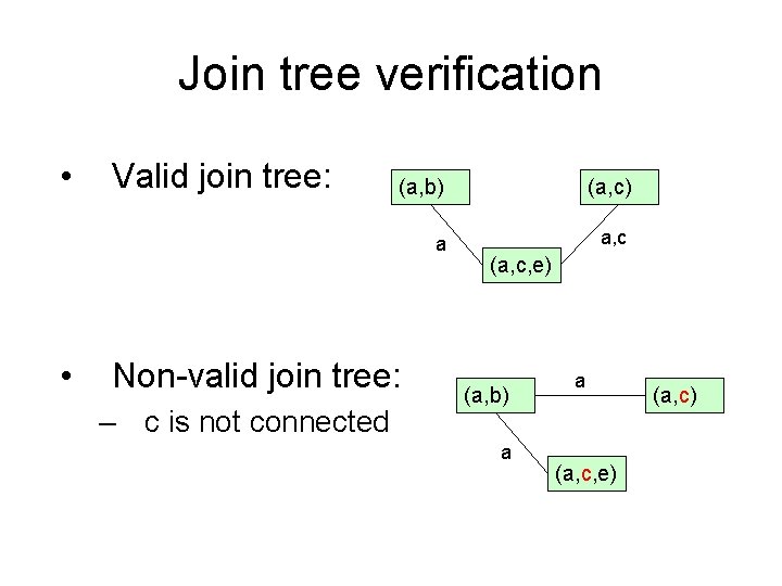
Join tree verification • • Valid join tree: (a, b) (a, c) a a, c Non-valid join tree: – c is not connected (a, c, e) (a, b) a a (a, c, e) (a, c)
Finding the join tree • There are several methods for finding the join tree (if there is one) • Some methods are based on the primal graph • We will see a method that is based on the dual graph
Finding a join tree for H • Algorithm JT-dual: 1. Compute the dual graph D(H) 2. Assign weights to edges: – The weight of each edge is the number of variables it represents 3. Compute the MST of the weighted graph – Denote the tree by T 4. If T is a valid joint tree, return T, Otherwise FAIL.
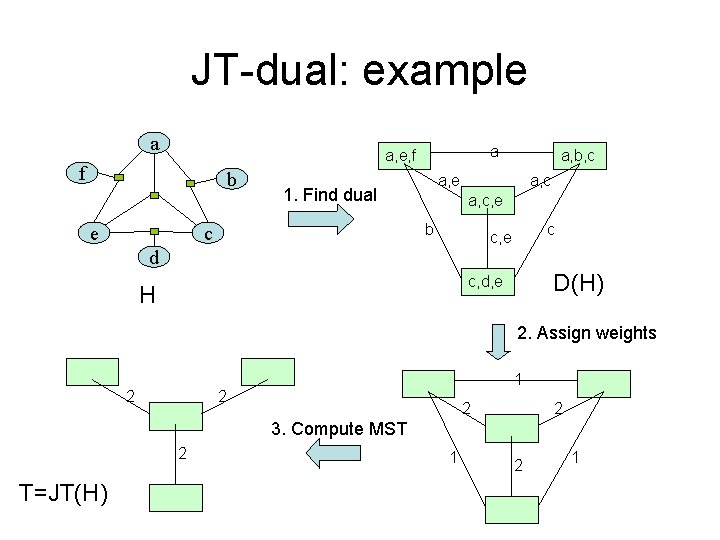
JT-dual: example a a a, e, f f b a, e 1. Find dual a, c, e b c e a, b, c c c, e d D(H) c, d, e H 2. Assign weights 2 1 2 2 2 3. Compute MST 2 T=JT(H) 1 2 1
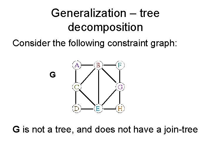
Generalization – tree decomposition Consider the following constraint graph: G G is not a tree, and does not have a join-tree
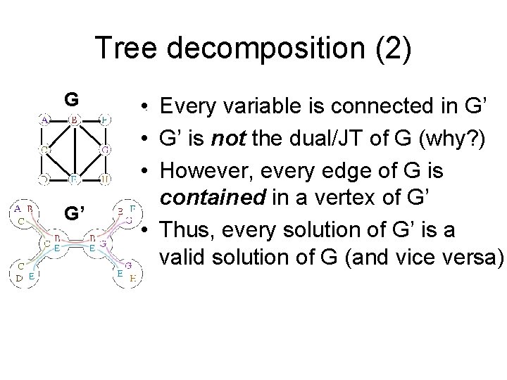
Tree decomposition (2) G G’ • Every variable is connected in G’ • G’ is not the dual/JT of G (why? ) • However, every edge of G is contained in a vertex of G’ • Thus, every solution of G’ is a valid solution of G (and vice versa)
Tree decomposition (3) • A graph TD(H) is called a tree decomposition of H if the following hold: – TD(H) is a tree – Every hyperedge of H is contained in a vertex of TD(H) – All nodes of TD(H) that contain the same variable are connected • What can we say about JT(H)?
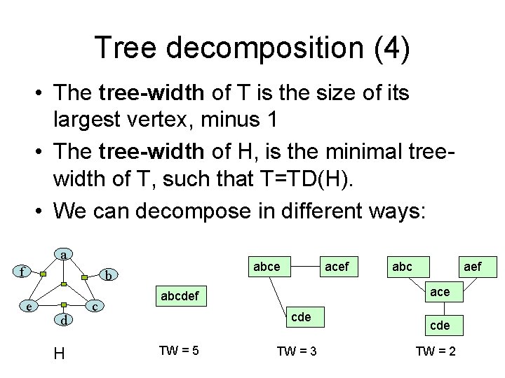
Tree decomposition (4) • The tree-width of T is the size of its largest vertex, minus 1 • The tree-width of H, is the minimal treewidth of T, such that T=TD(H). • We can decompose in different ways: a f abce b e d H c acef ace abcdef cde TW = 5 abc TW = 3 cde TW = 2
Bounded tree-width Theorem (Bodlaender 1996; Gottlob, Leone, and Scarcello 2000) For every fixed k, there is a polynomial time algorithm that: (a) Checks whether TW(H) ≤ k (b) If TW(H) ≤ k, returns a solution to H, or answers that such solution does not exist. The runtime of the algorithm is exponential in k.
- Slides: 50