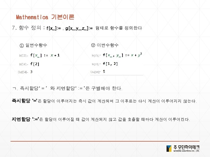
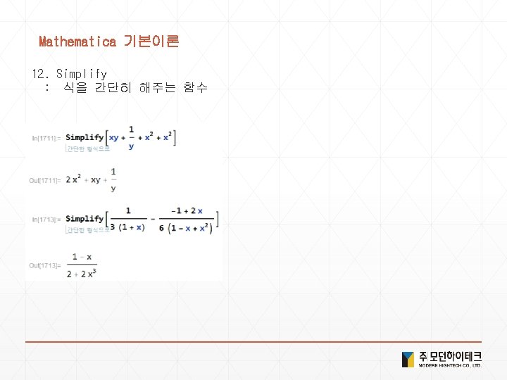
Mathematica Mathematica Palettes Classroom Assistant Mathematica Palettes Classroom


![Mathematica 기본이론 -Note- Wolfram 언어의 사칙연산 함수를 통해서도 계산이 가능하다. 2+2 : Plus[2, 2]](https://slidetodoc.com/presentation_image_h/9d503e106b8f7cdf69f9ad79f0b3eeec/image-26.jpg "Mathematica 기본이론 -Note- Wolfram 언어의 사칙연산 함수를 통해서도 계산이 가능하다. 2+2 : Plus[2, 2]")


![Mathematica 기본이론 11. N[ ] : 수치계산 / NSolve[ ]](https://slidetodoc.com/presentation_image_h/9d503e106b8f7cdf69f9ad79f0b3eeec/image-36.jpg "Mathematica 기본이론 11. N[ ] : 수치계산 / NSolve[ ]")


![Mathematica 기본이론 -Note- Wolfram 언어의 사칙연산 함수를 통해서도 계산이 가능하다. 2+2 : Plus[2, 2]](https://slidetodoc.com/presentation_image_h/9d503e106b8f7cdf69f9ad79f0b3eeec/image-81.jpg "Mathematica 기본이론 -Note- Wolfram 언어의 사칙연산 함수를 통해서도 계산이 가능하다. 2+2 : Plus[2, 2]")


![Mathematica 기본이론 11. N[ ] : 수치계산 / NSolve[ ]](https://slidetodoc.com/presentation_image_h/9d503e106b8f7cdf69f9ad79f0b3eeec/image-91.jpg "Mathematica 기본이론 11. N[ ] : 수치계산 / NSolve[ ]")


")


![Solution 1. 기초산술 1) 1234+5678 2) 1234*5678 3) 100/4 4) Plus[1234, 5678] , Times[1234,](https://slidetodoc.com/presentation_image_h/9d503e106b8f7cdf69f9ad79f0b3eeec/image-149.jpg "Solution 1. 기초산술 1) 1234+5678 2) 1234*5678 3) 100/4 4) Plus[1234, 5678] , Times[1234,")
![Solution 2. 함수정의 1) f[x_]: = x^2 2) value=Random. Color[] , value: =Random. Color[]](https://slidetodoc.com/presentation_image_h/9d503e106b8f7cdf69f9ad79f0b3eeec/image-150.jpg "Solution 2. 함수정의 1) f[x_]: = x^2 2) value=Random. Color[] , value: =Random. Color[]")
![Solution 3. Module 1) Module[{x = Range[10]}, x^2 + x] 2) Module[{x = Random.](https://slidetodoc.com/presentation_image_h/9d503e106b8f7cdf69f9ad79f0b3eeec/image-151.jpg "Solution 3. Module 1) Module[{x = Range[10]}, x^2 + x] 2) Module[{x = Random.")
![Solution 5. Date 생성 1) Table[5, 10] 2) Table[n + 1, {n, 1, 10}]](https://slidetodoc.com/presentation_image_h/9d503e106b8f7cdf69f9ad79f0b3eeec/image-152.jpg "Solution 5. Date 생성 1) Table[5, 10] 2) Table[n + 1, {n, 1, 10}]")
![Solution 6. Options 1) List. Plot[Table[x^2 + x, {x, 0, 10}], Plot. Theme ->](https://slidetodoc.com/presentation_image_h/9d503e106b8f7cdf69f9ad79f0b3eeec/image-153.jpg "Solution 6. Options 1) List. Plot[Table[x^2 + x, {x, 0, 10}], Plot. Theme ->")
 List. Line. Plot[Table[x^n, {n, 2, 4}, {x, 1,")
![Solution 8. Manipulate 1) Manipulate[List. Plot[Range[n]], {n, 5, 50, 1}] 2) Manipulate[Column[Table[a, n]], {n,](https://slidetodoc.com/presentation_image_h/9d503e106b8f7cdf69f9ad79f0b3eeec/image-155.jpg "Solution 8. Manipulate 1) Manipulate[List. Plot[Range[n]], {n, 5, 50, 1}] 2) Manipulate[Column[Table[a, n]], {n,")
![Solution 9. 대학수학 1) Limit[(x^2+5^x)/(x^2+2 x), x->0] Plot[(x^2+5 x)/(x^2+2 x), {x, -2, 2}] 2)](https://slidetodoc.com/presentation_image_h/9d503e106b8f7cdf69f9ad79f0b3eeec/image-156.jpg "Solution 9. 대학수학 1) Limit[(x^2+5^x)/(x^2+2 x), x->0] Plot[(x^2+5 x)/(x^2+2 x), {x, -2, 2}] 2)")
- Slides: 156
Mathematica
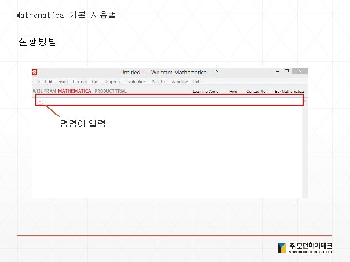
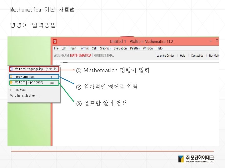
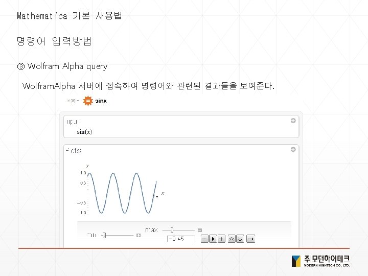
Mathematica 기본 사용법 명령어 입력방법 Palettes – Classroom Assistant
Mathematica 기본 사용법 명령어 입력방법 Palettes – Classroom Assistant
Mathematica 기본 사용법 명령어 입력방법 Palettes – Classroom Assistant
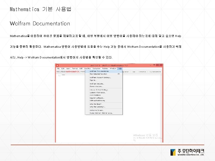
Mathematica 기본 사용법 Wolfram Documentation 검 색
Mathematica 기본 사용법 Wolfram Documentation
Mathematica 기본 사용법 Wolfram Documentation
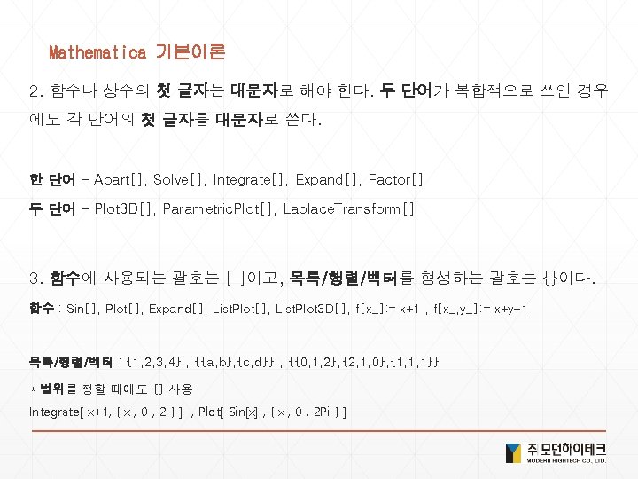
Mathematica 기본이론 소개
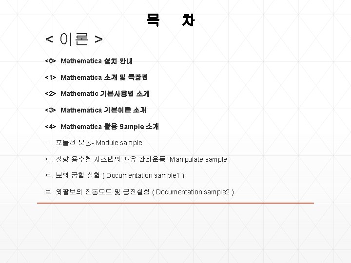
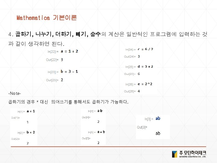
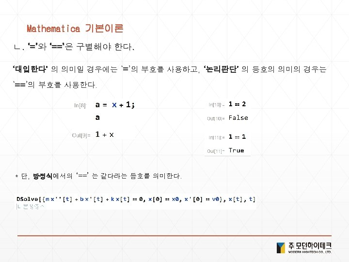
Mathematica 기본이론 -Note- Wolfram 언어의 사칙연산 함수를 통해서도 계산이 가능하다. 2+2 : Plus[2, 2] 5 -2 : Subtract[5, 2] 2*3 : Times[2, 3] 6/2 : Divide[6, 2] 3^2 : Power[3, 2] 최대값 : Max[3, 4] 최소값 : Min[3, 4] 무작위 자연수 : Random. Interger[ ]
Mathematica 기본이론 9. 단축키 : Ctrl + ^ : Esc + ee + Esc : Esc+ z/x/c + Esc : Ctrl + / : Esc + a/b/g + Esc : Esc + n/m/l +Esc : Ctrl + 2 : Esc + q/w/t + Esc : Esc + f/p/d + Esc : Ctrl + - : Esc + e + Esc : Esc + r/s/h + Esc : Esc + int + Esc : Esc + dd + Esc 이동 : Ctrl+Space 10. 값 초기화 ① 방법 1 : 함수(변수) =. ② 방법 2 : Clear[함수(변수)]
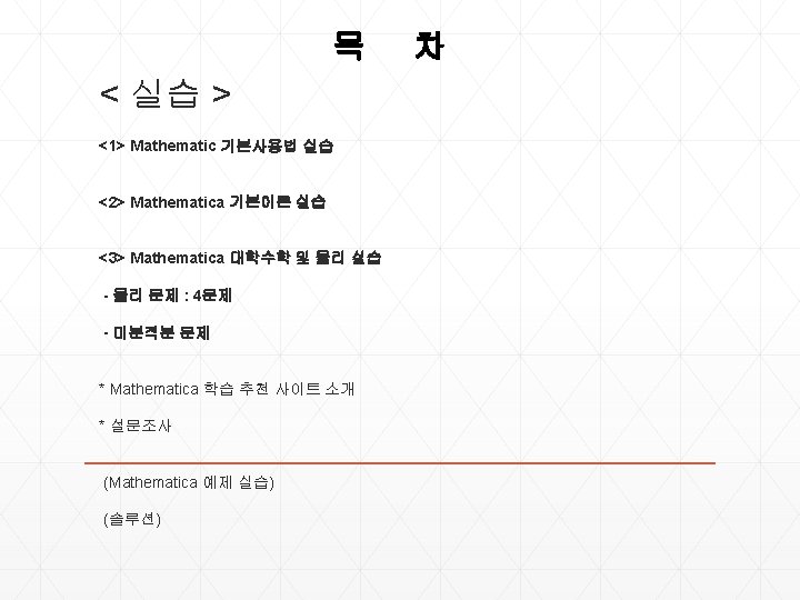
Mathematica 기본이론 11. N[ ] : 수치계산 / NSolve[ ]
Mathematica 기본이론 13. Import / Export * Import
Mathematica 기본이론 13. Import / Export * Export
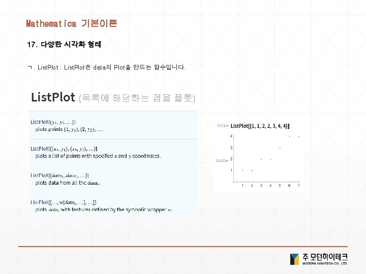
Mathematica 기본이론 17. 다양한 시각화 형태 ㄴ. List. Line. Plot
Mathematica 기본이론 17. 다양한 시각화 형태 ㄷ. Histogram & Pie. Chart
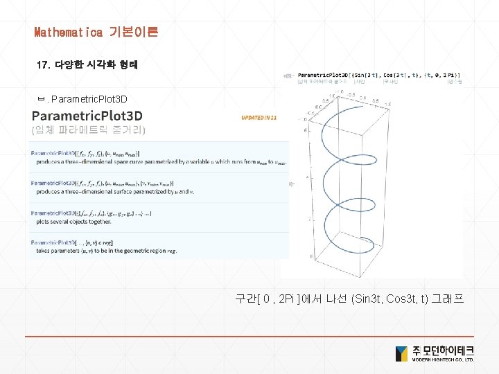
Mathematica 기본이론 17. 다양한 시각화 형태 ㄹ. Plot 3 D & List. Plot 3 D
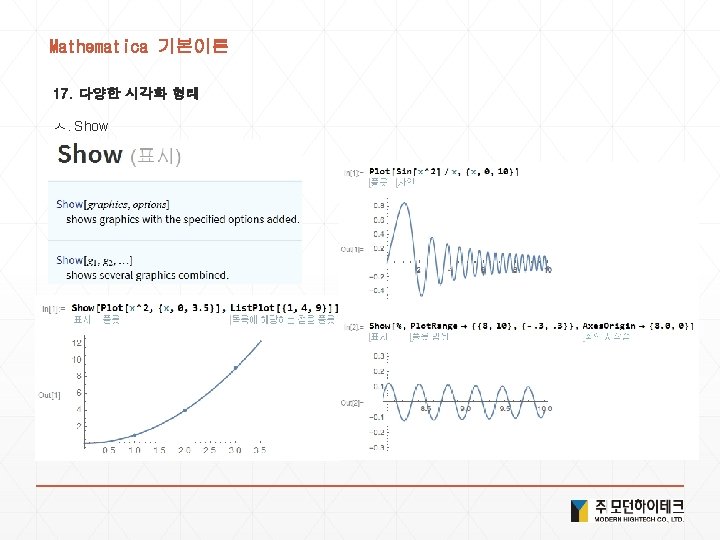
Mathematica 기본이론 17. 다양한 시각화 형태 ㅁ. Graphics & Graphics 3 D
MATHEMATICA 활용 SAMPLE 소개 ㄱ. 포물선 운동- Module sample ㄴ. 질량 용수철 시스템의 자유 감쇠운동- Manipulate sample ㄷ. 보의 굽힘 실험 -Documentation sample 1 ㄹ. 외팔보의 진동모드 및 공진실험 -Documentation sample 2
Mathematica 기본 사용법 명령어 입력방법 Palettes – Classroom Assistant
Mathematica 기본 사용법 명령어 입력방법 Palettes – Classroom Assistant
Mathematica 기본 사용법 명령어 입력방법 Palettes – Classroom Assistant
Mathematica 기본 사용법 Wolfram Documentation 검 색
Mathematica 기본 사용법 Wolfram Documentation
Mathematica 기본 사용법 Wolfram Documentation
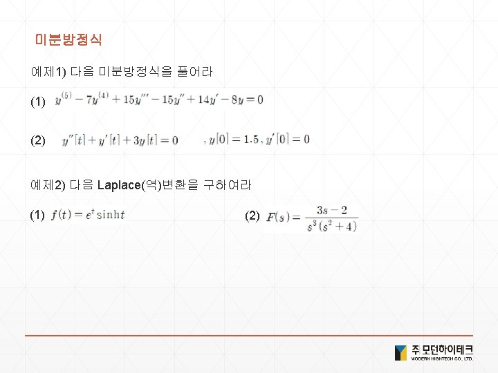
Mathematica 기본이론 실습
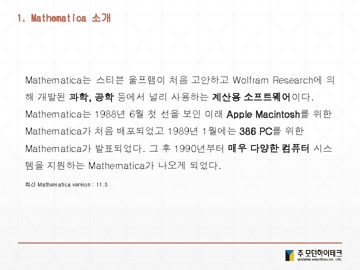
Mathematica 기본이론 -Note- Wolfram 언어의 사칙연산 함수를 통해서도 계산이 가능하다. 2+2 : Plus[2, 2] 5 -2 : Subtract[5, 2] 2*3 : Times[2, 3] 6/2 : Divide[6, 2] 3^2 : Power[3, 2] 최대값 : Max[3, 4] 최소값 : Min[3, 4] 무작위 자연수 : Random. Interger[ ]
Mathematica 기본이론 9. 단축키 : Ctrl + ^ : Esc + ee + Esc : Esc+ z/x/c + Esc : Ctrl + / : Esc + a/b/g + Esc : Esc + n/m/l +Esc : Ctrl + 2 : Esc + q/w/t + Esc : Esc + f/p/d + Esc : Ctrl + - : Esc + e + Esc : Esc + r/s/h + Esc : Esc + int + Esc : Esc + dd + Esc 이동 : Ctrl+Space 10. 값 초기화 ① 방법 1 : 함수(변수) =. ② 방법 2 : Clear[함수(변수)]
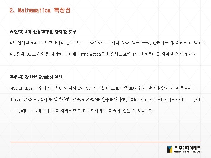
Mathematica 기본이론 11. N[ ] : 수치계산 / NSolve[ ]
Mathematica 기본이론 13. Import / Export * Import
Mathematica 기본이론 13. Import / Export * Export
Mathematica 기본이론 17. 다양한 시각화 형태 ㄴ. List. Line. Plot
Mathematica 기본이론 17. 다양한 시각화 형태 ㄷ. Histogram & Pie. Chart
Mathematica 기본이론 17. 다양한 시각화 형태 ㄹ. Plot 3 D & List. Plot 3 D
Mathematica 기본이론 17. 다양한 시각화 형태 ㅁ. Graphics & Graphics 3 D
MATHEMATICA 실습 - 물리 Mathematica 실습 – 4문제 - 미분적분 Mathematica 실습
* Mathematica 학습 추천 사이트 - http: //www. wolfram. com/mathematica ( Mathematica 사이트 ) - http: //demonstrations. wolfram. com/index. php (각종 학습소스) - http: //www. wolfram. com/wolfram-u/ (학습영상) - http: //community. wolfram. com/? source=footer (커뮤니티 게시판)
Mathematica 예제실습
S o l u t i o n
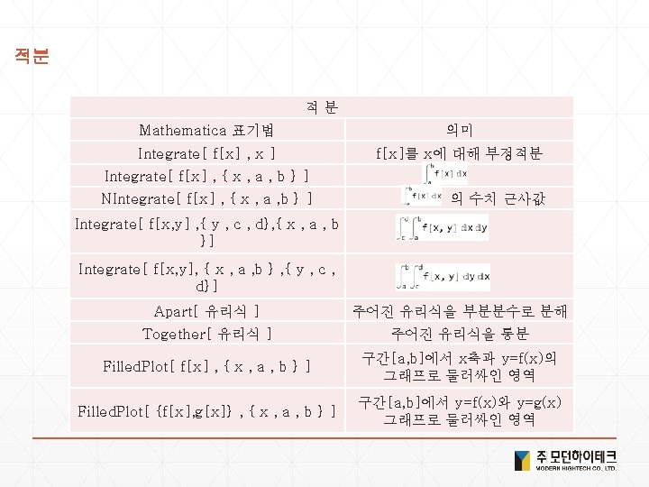
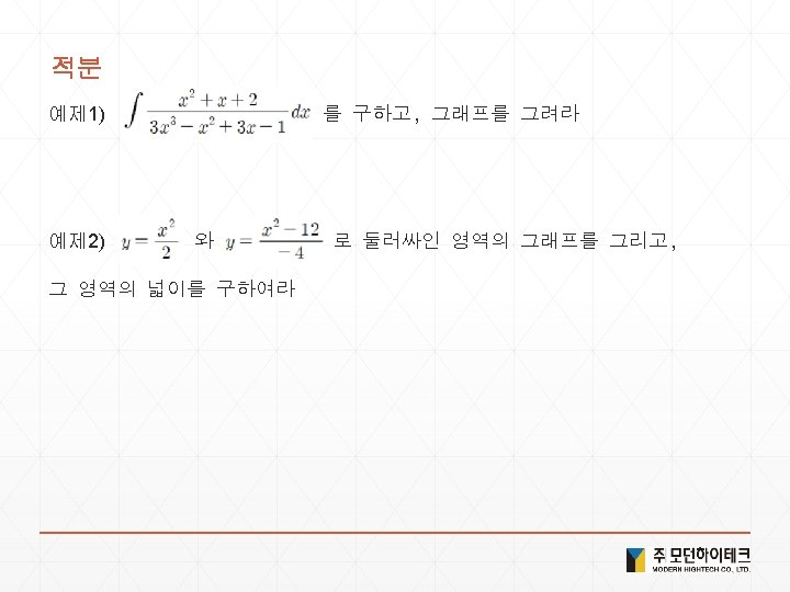
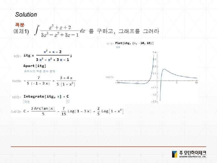
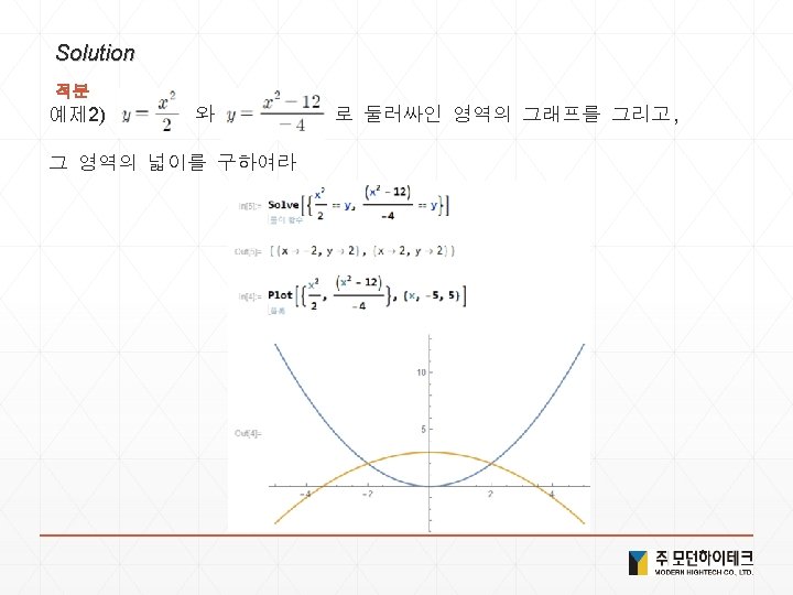
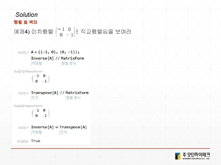
Solution 적분
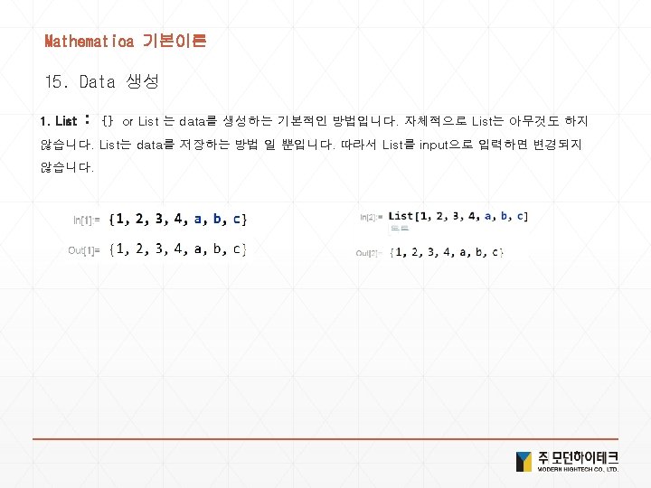
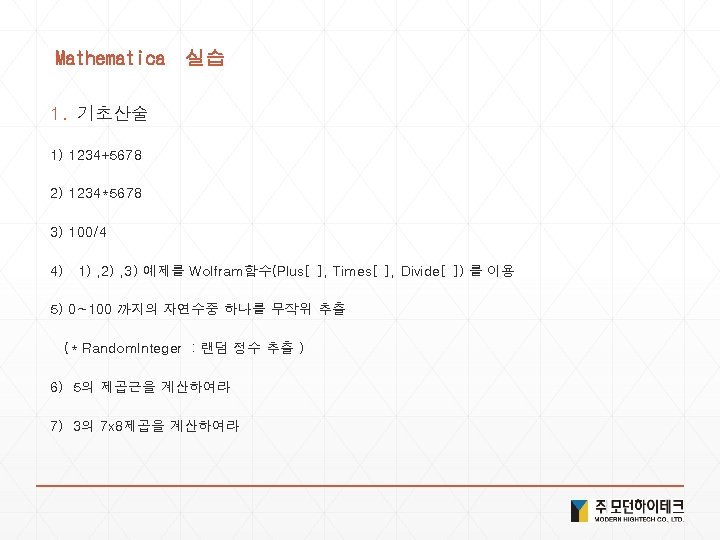
Solution 1. 기초산술 1) 1234+5678 2) 1234*5678 3) 100/4 4) Plus[1234, 5678] , Times[1234, 5678] , Divide[100, 4] 5) Random. Integer[100] 6) 5^2 7) 3^(7*8)
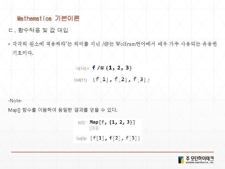
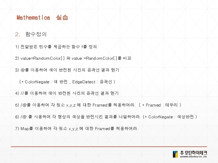
Solution 2. 함수정의 1) f[x_]: = x^2 2) value=Random. Color[] , value: =Random. Color[] 3) Color. Negate @ Edge. Detect @ 사진 4) 사진 // Edge. Detect // Color. Negate 5) Framed /@ {x, y, z} 6) Color. Negate /@ Entity. Value[ <Ctrl+ = planets> , "Image" ] 7) Map[Framed, {x, y, z}] 8) f[x_, y_] : = (x*y)/(x + y) 9) f[{a_, b_}] : = {a + b, a - b, a*b} 10) x//d//c//b//a 11) Framed /@ Alphabet[] 12) Map[Framed, Alphabet[]] 13) Geo. Graphics /@ Entity. List[ <Ctrl+ = countries in G 5> ] 14) Map[Geo. Graphics, Entity. List[ <Ctrl+ = countries in G 5> ]
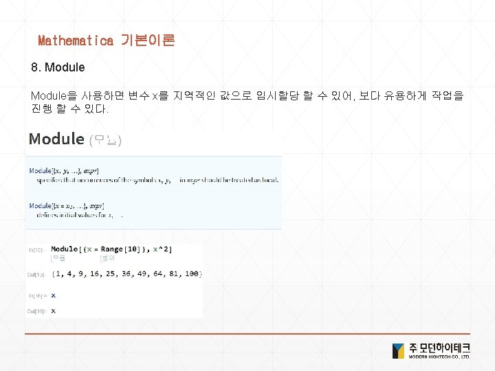
Solution 3. Module 1) Module[{x = Range[10]}, x^2 + x] 2) Module[{x = Random. Integer[100, 10]}, Column[{x, Sort[x], Max[x], Total[x]}]] 3) Module[{x = Range[10], n = 2}, x^n] 4) Module[{x, y}, x = Range[10]; y = x^2 ; y = y + 10000]
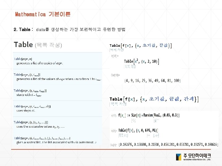
Solution 5. Date 생성 1) Table[5, 10] 2) Table[n + 1, {n, 1, 10}] 3) Table[Random. Integer[10], 20] 4) Table[2 n + 1, {n, 0, 49}] 5) Bar. Chart[Table[n^2, {n, 1, 10}]] 6) Table[n^2 + 2, {n, 10, 2}] 7) f[x_] : = Sin[x] + Cos[x] Table[f[x], {x, 0, 6 Pi, Pi}]
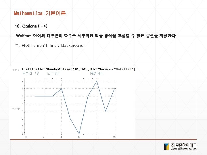
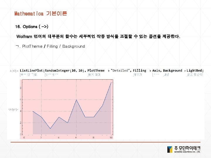
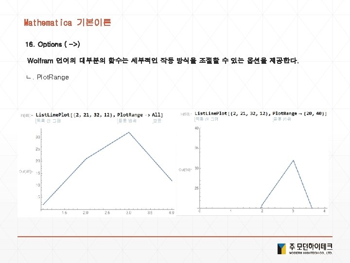
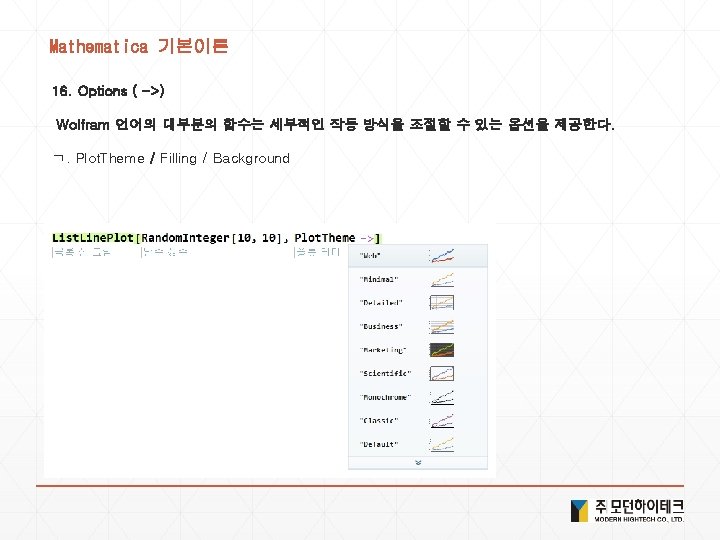
Solution 6. Options 1) List. Plot[Table[x^2 + x, {x, 0, 10}], Plot. Theme -> "Marketing"] 2) List. Plot[Table[x^2 + x, {x, 0, 10}], Filling -> Axis] 3) List. Plot[Table[x^2 + x, {x, 0, 10}], Background -> Yellow] 4) List. Plot[{1, 3, 2, 5, 4}, Plot. Range -> {{-1, 6}, {-1, 6}}] 5) Plot[{Sin[x], Sin[2 x], Sin[3 x]}, {x, 0, 2 Pi}, Plot. Style -> {{RGBColor[0. 5, 0. 5], RGBColor[0. 83, 0. 5], RGBColor[0. 5, 0. 16, 0. 5]}, Thickness[0. 01]}, Frame -> True]
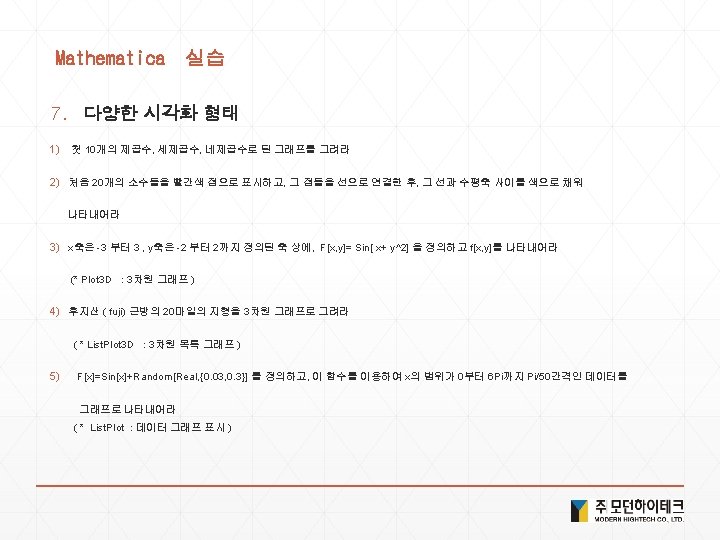
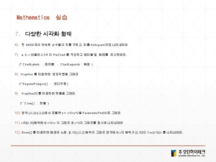
Solution 7. 다양한 시각화 형태 1) List. Line. Plot[Table[x^n, {n, 2, 4}, {x, 1, 10}]] 2) List. Line. Plot[Table[Prime[n], {n, 20}], Filling -> Axis, Mesh -> True, Mesh. Style -> Red] 3) f[x_, y_] : = Sin[x + y^2] Plot 3 D[f[x, y], {x, -3, 3}, {y, -2, 2}] 4) List. Plot 3 D[Geo. Elevation. Data[Geo. Disk[ <Ctrl+ = mount fuji>]]] 5) f[x_] : = Sin[x] + Random[Real, {0. 03, 0. 3}] List. Plot[Table[f[x], {x, 0, 6 Pi, Pi/50}]] 6) Histogram[Table[Prime[n + 1] - Prime[n], {n, 10000}]] 7) Pie. Chart[{2, 3, 5}, Chart. Labels -> {"a", "b", "c"}, Chart. Legends -> {"a", "b", "c"}] 8) Graphics[Regular. Polygon[5]] 9) Graphics 3 D[Cone[]] 10) Parametric. Plot 3 D[{x, y, x^2 + y^2}, {x, -2, 2}, {y, -2, 2}] 11) Show[ Plot[x^2 + x, {x, 0, 10}], Plot[x^3, {x, 0, 10}]] 12) Show[ Plot[Cos[x^2/x], {x, 2, 10}], Background -> Yellow, Plot. Range -> {{0, 10}, {-2, 2}}]
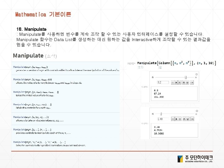
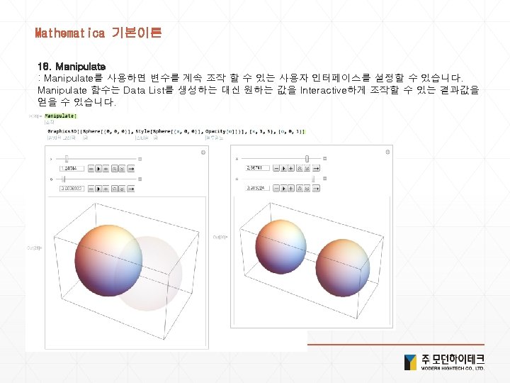
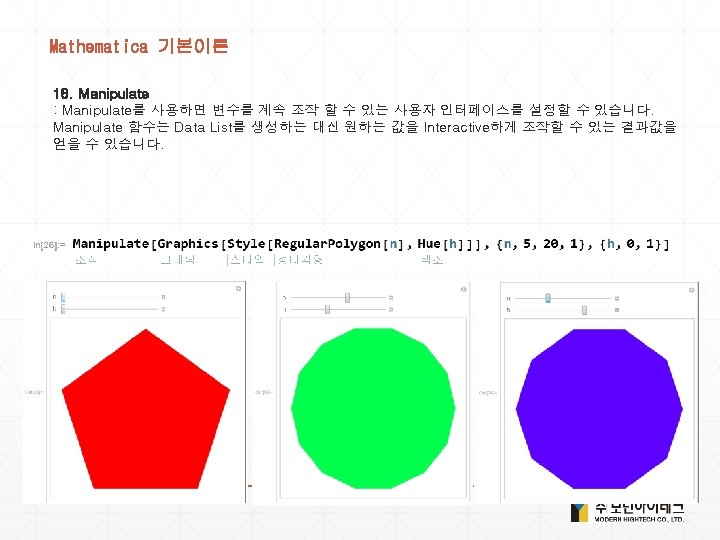
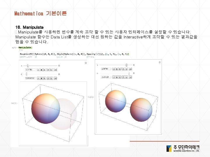
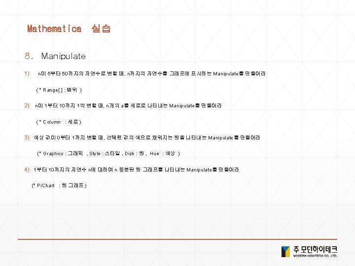
Solution 8. Manipulate 1) Manipulate[List. Plot[Range[n]], {n, 5, 50, 1}] 2) Manipulate[Column[Table[a, n]], {n, 1, 10, 1}] 3) Manipulate[Graphics[Style[Disk[], Hue[n]]], {n, 0, 1}] 4) Manipulate[Pie. Chart[Table[1, n]], {n, 1, 10, 1}]
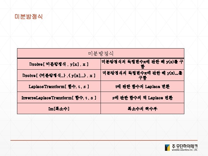
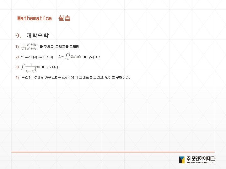
Solution 9. 대학수학 1) Limit[(x^2+5^x)/(x^2+2 x), x->0] Plot[(x^2+5 x)/(x^2+2 x), {x, -2, 2}] 2) For[i=0, i<=10, i++, s= ; Print["n=", i , “ -> ", s]] 3). 4) Plot[Floor[x], {x, -1, 5}, Filling->Axis]