Math Review with Matlab Laplace Transform Application Linear

Math Review with Matlab: Laplace Transform Application: Linear Time Invariant (LTI) Systems S. Awad, Ph. D. M. Corless, M. S. E. E. E. C. E. Department University of Michigan-Dearborn

X(s) Laplace Transform: Linear Time Invariant Systems Linear Time Invariant (LTI) Systems § § § § Definition of a Linear Time Invariant System Impulse Response Transfer Function Simple Systems Simple System Example Pulse Response Example Transient and Steady State Example 2

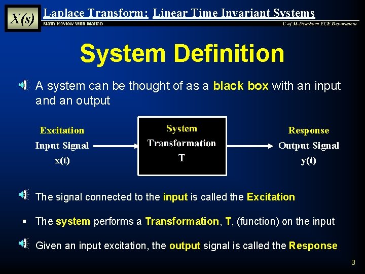
X(s) Laplace Transform: Linear Time Invariant Systems System Definition § A system can be thought of as a black box with an input and an output Excitation Input Signal x(t) Response Output Signal y(t) § The signal connected to the input is called the Excitation § The system performs a Transformation, T, (function) on the input § Given an input excitation, the output signal is called the Response 3

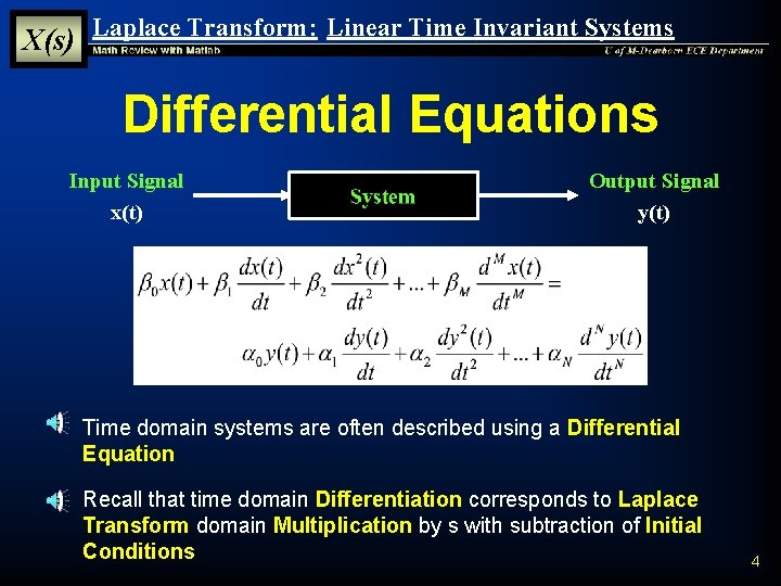
X(s) Laplace Transform: Linear Time Invariant Systems Differential Equations Input Signal x(t) Output Signal y(t) § Time domain systems are often described using a Differential Equation § Recall that time domain Differentiation corresponds to Laplace Transform domain Multiplication by s with subtraction of Initial Conditions 4

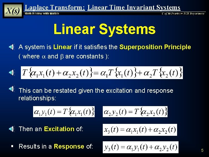
X(s) Laplace Transform: Linear Time Invariant Systems Linear Systems § A system is Linear if it satisfies the Superposition Principle ( where a and b are constants ): § This can be restated given the excitation and response relationships: § Then an Excitation of: § Results in a Response of: 5

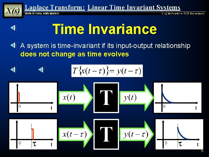
X(s) Laplace Transform: Linear Time Invariant Systems Time Invariance § A system is time-invariant if its input-output relationship does not change as time evolves 0 0 t t t 6

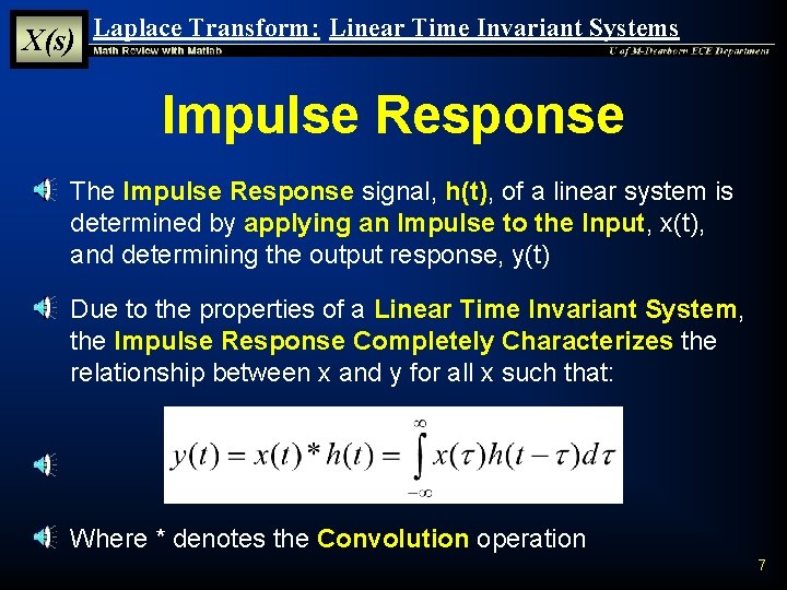
X(s) Laplace Transform: Linear Time Invariant Systems Impulse Response § The Impulse Response signal, h(t), of a linear system is determined by applying an Impulse to the Input, x(t), and determining the output response, y(t) § Due to the properties of a Linear Time Invariant System, the Impulse Response Completely Characterizes the relationship between x and y for all x such that: § Where * denotes the Convolution operation 7

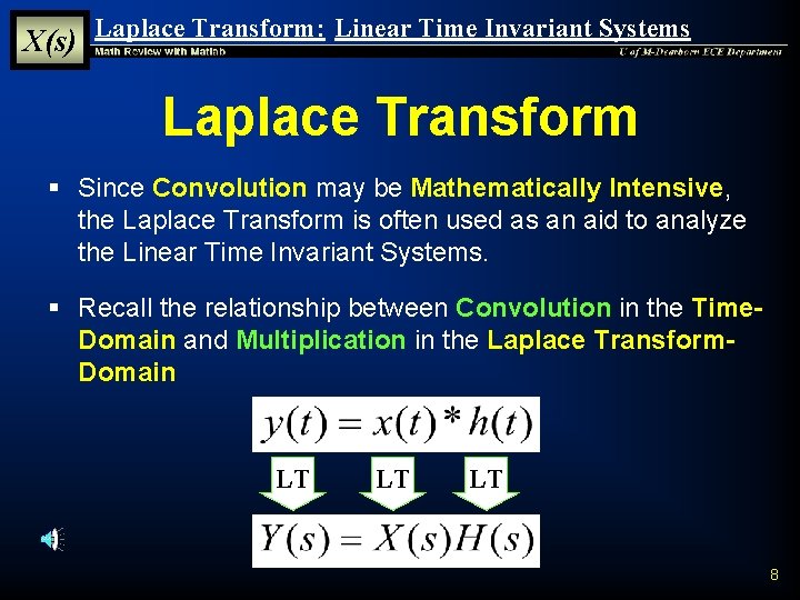
X(s) Laplace Transform: Linear Time Invariant Systems Laplace Transform § Since Convolution may be Mathematically Intensive, the Laplace Transform is often used as an aid to analyze the Linear Time Invariant Systems. § Recall the relationship between Convolution in the Time. Domain and Multiplication in the Laplace Transform. Domain LT LT LT 8

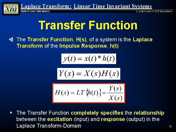
X(s) Laplace Transform: Linear Time Invariant Systems Transfer Function § The Transfer Function, H(s), of a system is the Laplace Transform of the Impulse Response, h(t) § The Transfer Function completely specifies the relationship between the excitation (input) and response (output) in the Laplace Transform-Domain 9

X(s) Laplace Transform: Linear Time Invariant Systems Simple Systems § Most systems can be created by combining the following simple system building blocks: § Linear Operations: u Multiplication by a Constant u Addition of Signals § Time-Domain Differentiation § Time-Domain Integration § Time-Domain Delay 10

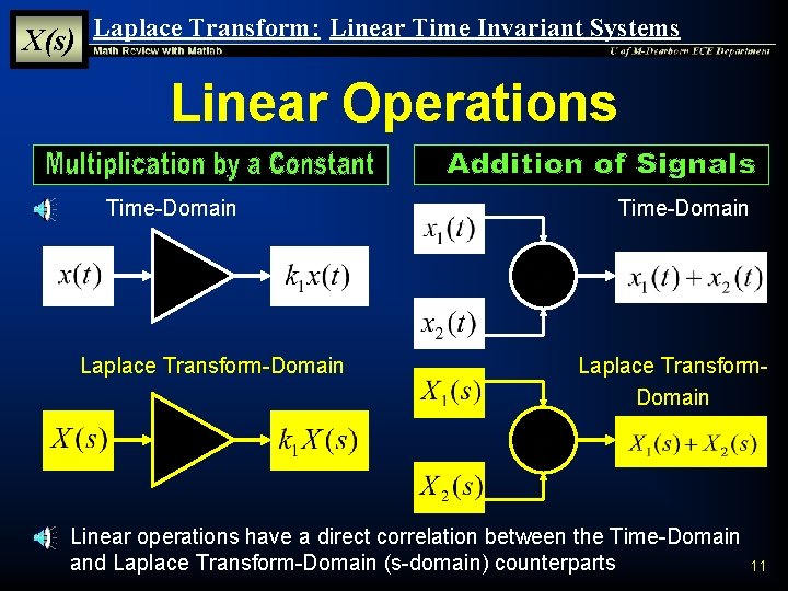
X(s) Laplace Transform: Linear Time Invariant Systems Linear Operations Time-Domain Laplace Transform-Domain Time-Domain Laplace Transform. Domain § Linear operations have a direct correlation between the Time-Domain and Laplace Transform-Domain (s-domain) counterparts 11

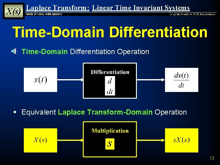
X(s) Laplace Transform: Linear Time Invariant Systems Time-Domain Differentiation § Time-Domain Differentiation Operation § Equivalent Laplace Transform-Domain Operation 12

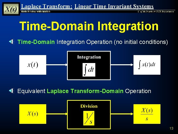
X(s) Laplace Transform: Linear Time Invariant Systems Time-Domain Integration § Time-Domain Integration Operation (no initial conditions) § Equivalent Laplace Transform-Domain Operation 13

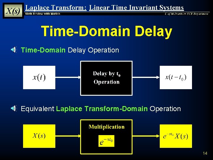
X(s) Laplace Transform: Linear Time Invariant Systems Time-Domain Delay § Time-Domain Delay Operation § Equivalent Laplace Transform-Domain Operation 14

X(s) Laplace Transform: Linear Time Invariant Systems Examples of LTI Systems § The building blocks described previously can be used to model and analyze real world systems such as: § Audio Equalizers (band pass filters) § Automatic Gain Controls for a radio § Car Mufflers (mechanical filter) § Suspension Systems (mechanical low pass filter) § Cruise Control (motor speed control) 15

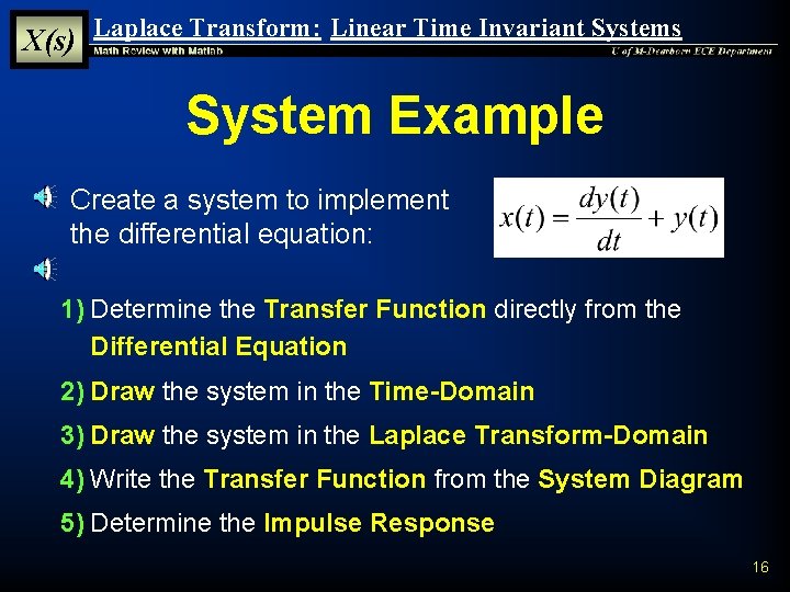
X(s) Laplace Transform: Linear Time Invariant Systems System Example § Create a system to implement the differential equation: 1) Determine the Transfer Function directly from the Differential Equation 2) Draw the system in the Time-Domain 3) Draw the system in the Laplace Transform-Domain 4) Write the Transfer Function from the System Diagram 5) Determine the Impulse Response 16

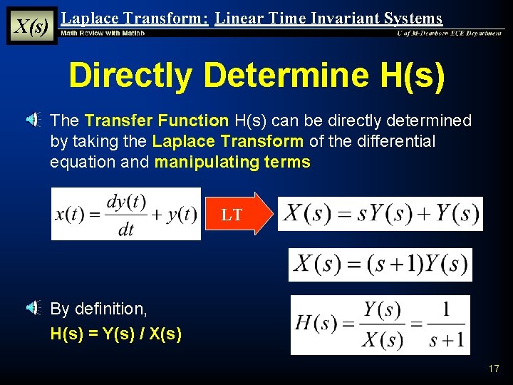
X(s) Laplace Transform: Linear Time Invariant Systems Directly Determine H(s) § The Transfer Function H(s) can be directly determined by taking the Laplace Transform of the differential equation and manipulating terms LT § By definition, H(s) = Y(s) / X(s) 17

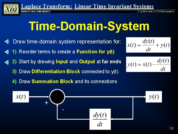
X(s) Laplace Transform: Linear Time Invariant Systems Time-Domain-System § Draw time-domain system representation for: 1) Reorder terms to create a Function for y(t) 2) Start by drawing Input and Output at far ends 3) Draw Differentiation Block connected to y(t) 4) Draw Summation Block and its connections + 18

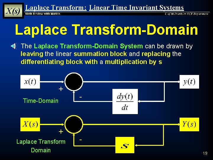
X(s) Laplace Transform: Linear Time Invariant Systems Laplace Transform-Domain § The Laplace Transform-Domain System can be drawn by leaving the linear summation block and replacing the differentiating block with a multiplication by s + Time-Domain + Laplace Transform Domain - 19

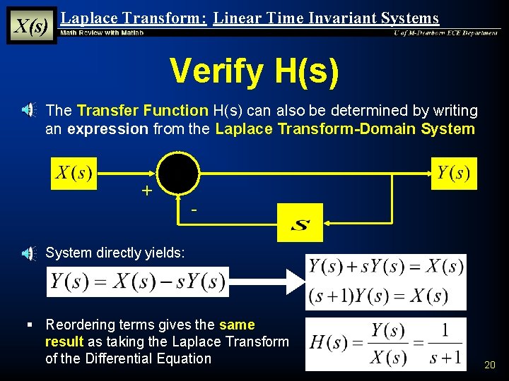
X(s) Laplace Transform: Linear Time Invariant Systems Verify H(s) § The Transfer Function H(s) can also be determined by writing an expression from the Laplace Transform-Domain System + - § System directly yields: § Reordering terms gives the same result as taking the Laplace Transform of the Differential Equation 20

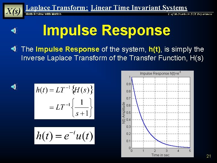
X(s) Laplace Transform: Linear Time Invariant Systems Impulse Response § The Impulse Response of the system, h(t), is simply the Inverse Laplace Transform of the Transfer Function, H(s) 21

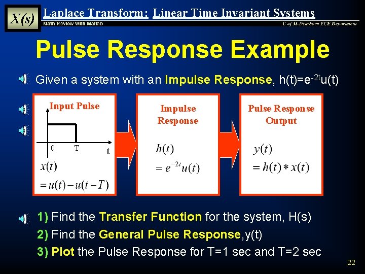
X(s) Laplace Transform: Linear Time Invariant Systems Pulse Response Example § Given a system with an Impulse Response, h(t)=e-2 tu(t) Input Pulse 0 T Impulse Response Pulse Response Output t 1) Find the Transfer Function for the system, H(s) 2) Find the General Pulse Response, y(t) 3) Plot the Pulse Response for T=1 sec and T=2 sec 22

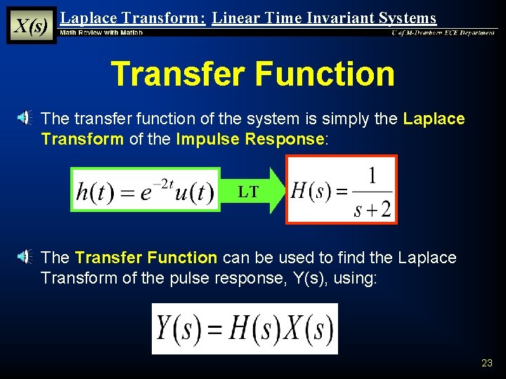
X(s) Laplace Transform: Linear Time Invariant Systems Transfer Function § The transfer function of the system is simply the Laplace Transform of the Impulse Response: LT § The Transfer Function can be used to find the Laplace Transform of the pulse response, Y(s), using: 23

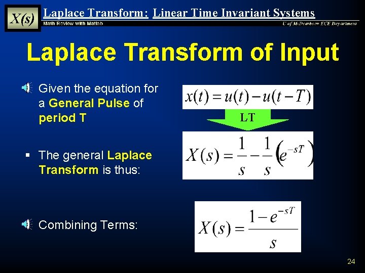
X(s) Laplace Transform: Linear Time Invariant Systems Laplace Transform of Input § Given the equation for a General Pulse of period T LT § The general Laplace Transform is thus: § Combining Terms: 24

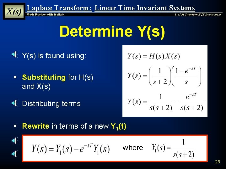
X(s) Laplace Transform: Linear Time Invariant Systems Determine Y(s) § Y(s) is found using: § Substituting for H(s) and X(s) § Distributing terms § Rewrite in terms of a new Y 1(t) where 25

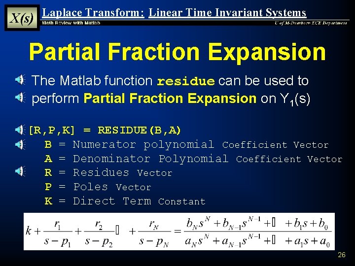
X(s) Laplace Transform: Linear Time Invariant Systems Partial Fraction Expansion § The Matlab function residue can be used to perform Partial Fraction Expansion on Y 1(s) [R, P, K] = RESIDUE(B, A) B = Numerator polynomial Coefficient Vector A = Denominator Polynomial Coefficient Vector R = Residues Vector P = Poles Vector K = Direct Term Constant 26

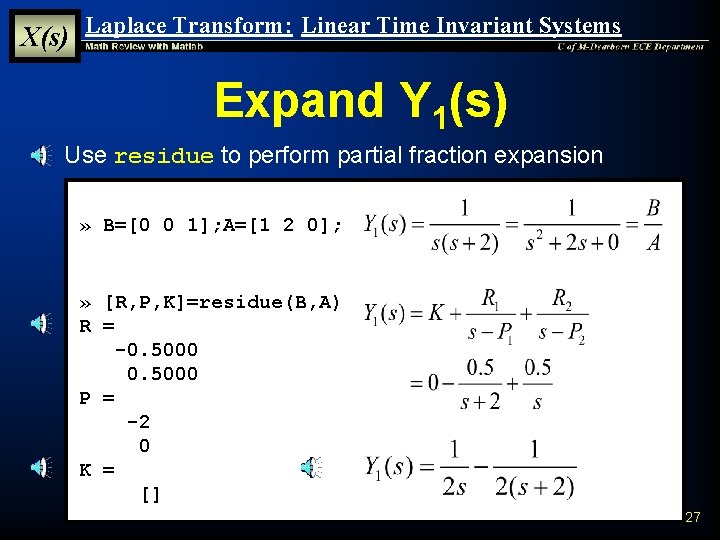
X(s) Laplace Transform: Linear Time Invariant Systems Expand Y 1(s) § Use residue to perform partial fraction expansion » B=[0 0 1]; A=[1 2 0]; » [R, P, K]=residue(B, A) R = -0. 5000 P = -2 0 K = [] 27

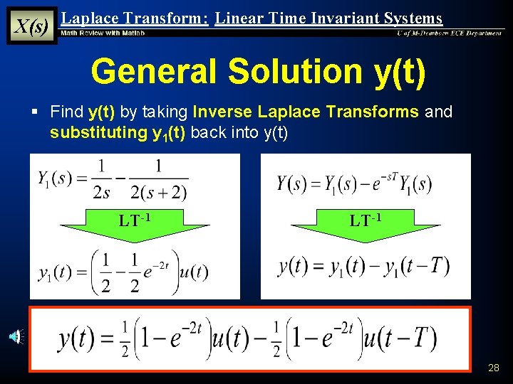
X(s) Laplace Transform: Linear Time Invariant Systems General Solution y(t) § Find y(t) by taking Inverse Laplace Transforms and substituting y 1(t) back into y(t) LT-1 28

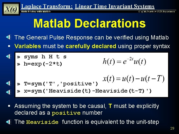
X(s) Laplace Transform: Linear Time Invariant Systems Matlab Declarations § The General Pulse Response can be verified using Matlab § Variables must be carefully declared using proper syntax » syms h H t s » h=exp(-2*t) » T=sym('T', 'positive') » x=sym('Heaviside(t)-Heaviside(t-T)') § Assuming the system to be causal, T must be explicitly declared as a positive number § The Heaviside function is equivalent to the unit-step 29

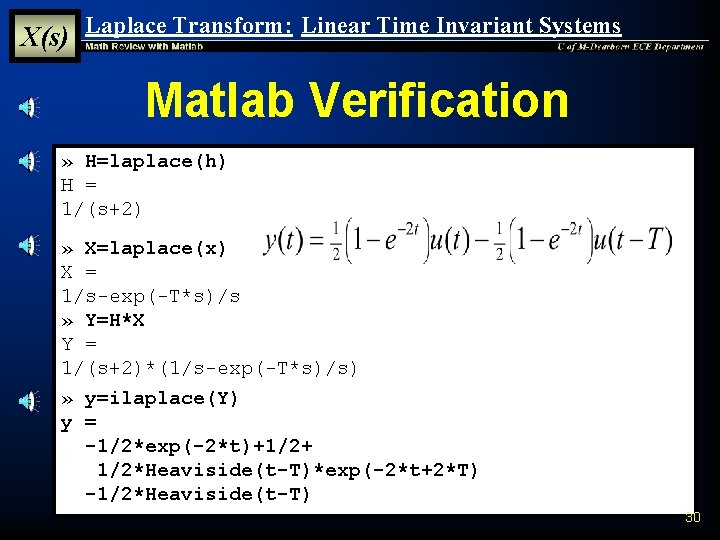
X(s) Laplace Transform: Linear Time Invariant Systems Matlab Verification » H=laplace(h) H = 1/(s+2) » X=laplace(x) X = 1/s-exp(-T*s)/s » Y=H*X Y = 1/(s+2)*(1/s-exp(-T*s)/s) » y=ilaplace(Y) y = -1/2*exp(-2*t)+1/2+ 1/2*Heaviside(t-T)*exp(-2*t+2*T) -1/2*Heaviside(t-T) 30

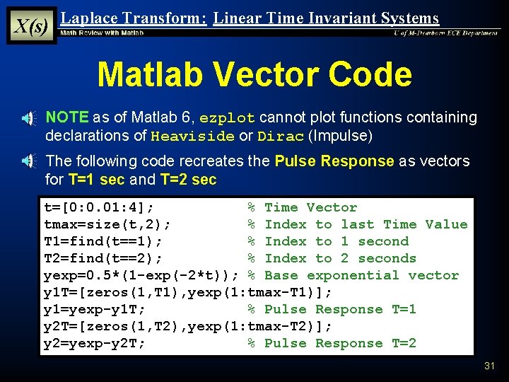
X(s) Laplace Transform: Linear Time Invariant Systems Matlab Vector Code § NOTE as of Matlab 6, ezplot cannot plot functions containing declarations of Heaviside or Dirac (Impulse) § The following code recreates the Pulse Response as vectors for T=1 sec and T=2 sec t=[0: 0. 01: 4]; % Time Vector tmax=size(t, 2); % Index to last Time Value T 1=find(t==1); % Index to 1 second T 2=find(t==2); % Index to 2 seconds yexp=0. 5*(1 -exp(-2*t)); % Base exponential vector y 1 T=[zeros(1, T 1), yexp(1: tmax-T 1)]; y 1=yexp-y 1 T; % Pulse Response T=1 y 2 T=[zeros(1, T 2), yexp(1: tmax-T 2)]; y 2=yexp-y 2 T; % Pulse Response T=2 31

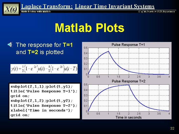
X(s) Laplace Transform: Linear Time Invariant Systems Matlab Plots § The response for T=1 and T=2 is plotted subplot(2, 1, 1); plot(t, y 1); title('Pulse Response T=1'); grid on; subplot(2, 1, 2); plot(t, y 2); title('Pulse Response T=2'); xlabel('Time in seconds'); grid on; 32

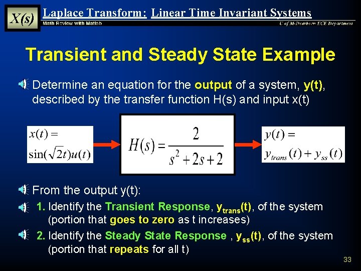
X(s) Laplace Transform: Linear Time Invariant Systems Transient and Steady State Example § Determine an equation for the output of a system, y(t), described by the transfer function H(s) and input x(t) § From the output y(t): 1. Identify the Transient Response, ytrans(t), of the system (portion that goes to zero as t increases) 2. Identify the Steady State Response , yss(t), of the system (portion that repeats for all t) 33

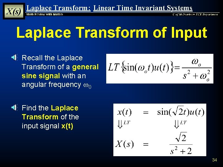
X(s) Laplace Transform: Linear Time Invariant Systems Laplace Transform of Input § Recall the Laplace Transform of a general sine signal with an angular frequency w 0 § Find the Laplace Transform of the input signal x(t) 34

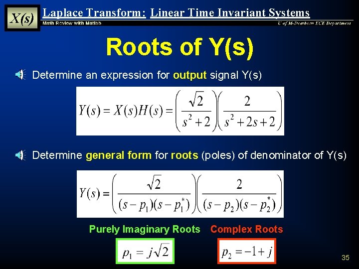
X(s) Laplace Transform: Linear Time Invariant Systems Roots of Y(s) § Determine an expression for output signal Y(s) § Determine general form for roots (poles) of denominator of Y(s) Purely Imaginary Roots Complex Roots 35

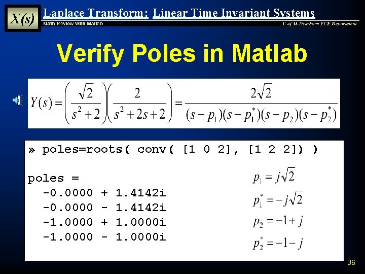
X(s) Laplace Transform: Linear Time Invariant Systems Verify Poles in Matlab » poles=roots( conv( [1 0 2], [1 2 2]) ) poles = -0. 0000 -1. 0000 + + - 1. 4142 i 1. 0000 i 36

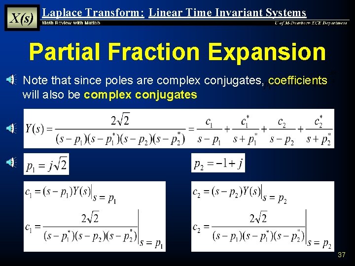
X(s) Laplace Transform: Linear Time Invariant Systems Partial Fraction Expansion § Note that since poles are complex conjugates, coefficients will also be complex conjugates 37

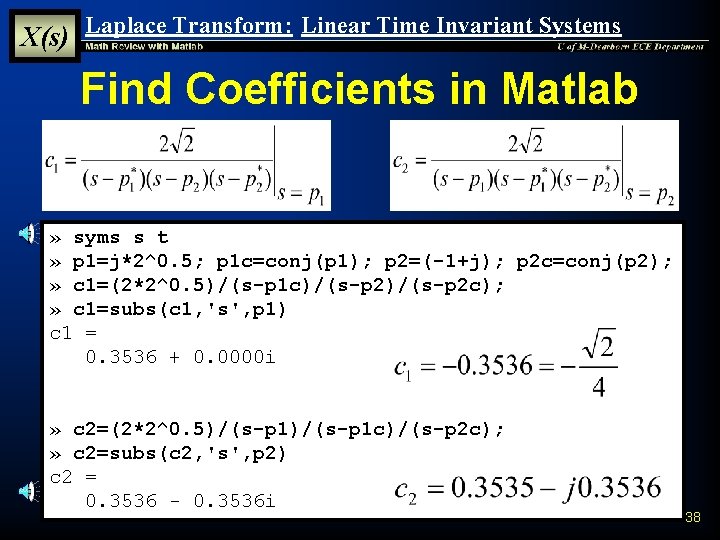
X(s) Laplace Transform: Linear Time Invariant Systems Find Coefficients in Matlab » syms s t » p 1=j*2^0. 5; p 1 c=conj(p 1); p 2=(-1+j); p 2 c=conj(p 2); » c 1=(2*2^0. 5)/(s-p 1 c)/(s-p 2 c); » c 1=subs(c 1, 's', p 1) c 1 = 0. 3536 + 0. 0000 i » c 2=(2*2^0. 5)/(s-p 1 c)/(s-p 2 c); » c 2=subs(c 2, 's', p 2) c 2 = 0. 3536 - 0. 3536 i 38

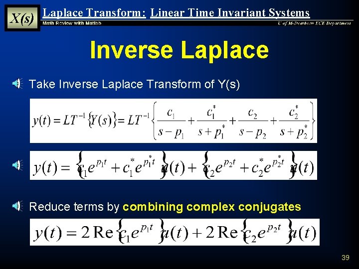
X(s) Laplace Transform: Linear Time Invariant Systems Inverse Laplace § Take Inverse Laplace Transform of Y(s) § Reduce terms by combining complex conjugates 39

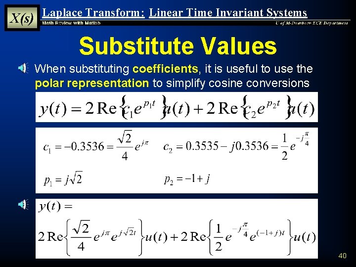
X(s) Laplace Transform: Linear Time Invariant Systems Substitute Values § When substituting coefficients, it is useful to use the polar representation to simplify cosine conversions 40

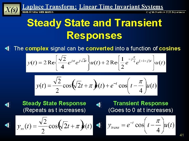
X(s) Laplace Transform: Linear Time Invariant Systems Steady State and Transient Responses § The complex signal can be converted into a function of cosines Steady State Response (Repeats as t increases) Transient Response (Goes to 0 at t increases) 41

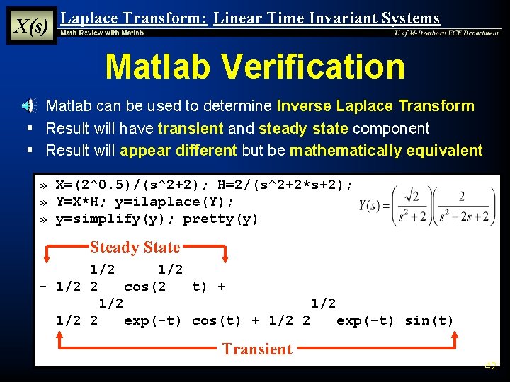
X(s) Laplace Transform: Linear Time Invariant Systems Matlab Verification § Matlab can be used to determine Inverse Laplace Transform § Result will have transient and steady state component § Result will appear different but be mathematically equivalent » X=(2^0. 5)/(s^2+2); H=2/(s^2+2*s+2); » Y=X*H; y=ilaplace(Y); » y=simplify(y); pretty(y) Steady State 1/2 - 1/2 2 cos(2 t) + 1/2 1/2 2 exp(-t) cos(t) + 1/2 2 exp(-t) sin(t) Transient 42

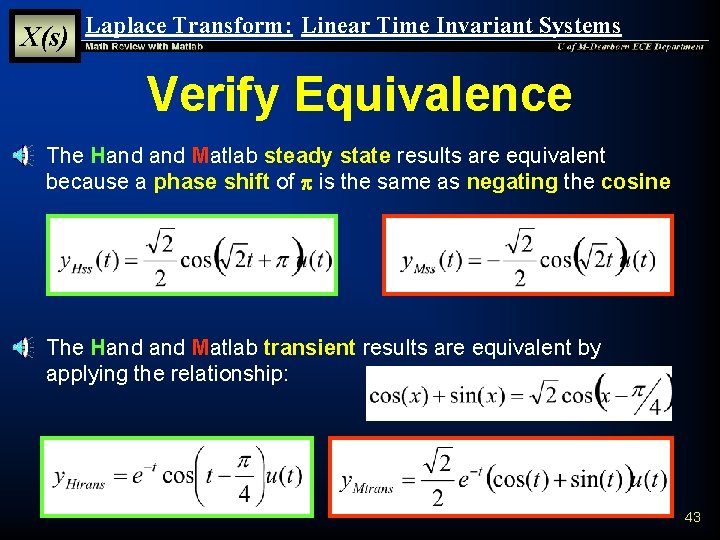
X(s) Laplace Transform: Linear Time Invariant Systems Verify Equivalence § The Hand Matlab steady state results are equivalent because a phase shift of p is the same as negating the cosine § The Hand Matlab transient results are equivalent by applying the relationship: 43

X(s) Laplace Transform: Linear Time Invariant Systems Summary § Laplace Transform is a useful technique for analyzing Linear Time Invariant Systems § Impulse Response and its Laplace Transform, the Transfer Function, are used to describe system characteristics § Simple System Blocks for multiplication, addition, differentiation, integration, and time shifting can be used to describe many real world systems § Matlab can be used to determine the Transient and Steady-State Responses of a complex system 44