MATH 2311 Help Using RStudio To download RStudio

MATH 2311 Help Using R-Studio

To download R-Studio Go to the following link: http: //cran. cnr. berkeley. edu/ and https: //www. rstudio. com/products/rstudio/download 3/ Follow the instructions for your computer operating system.

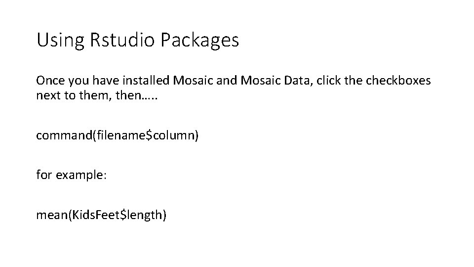
Using Rstudio Packages Once you have installed Mosaic and Mosaic Data, click the checkboxes next to them, then…. . command(filename$column) for example: mean(Kids. Feet$length)

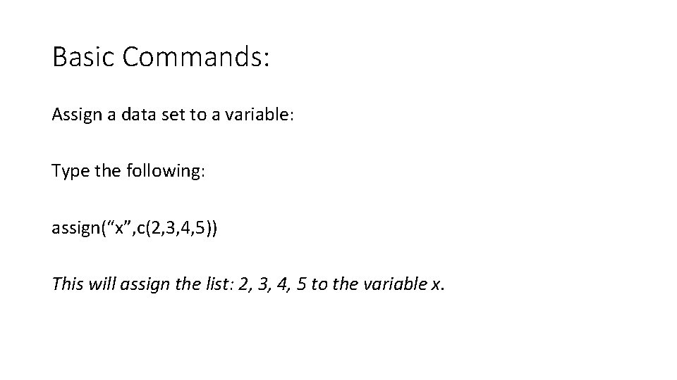
Basic Commands: Assign a data set to a variable: Type the following: assign(“x”, c(2, 3, 4, 5)) This will assign the list: 2, 3, 4, 5 to the variable x.

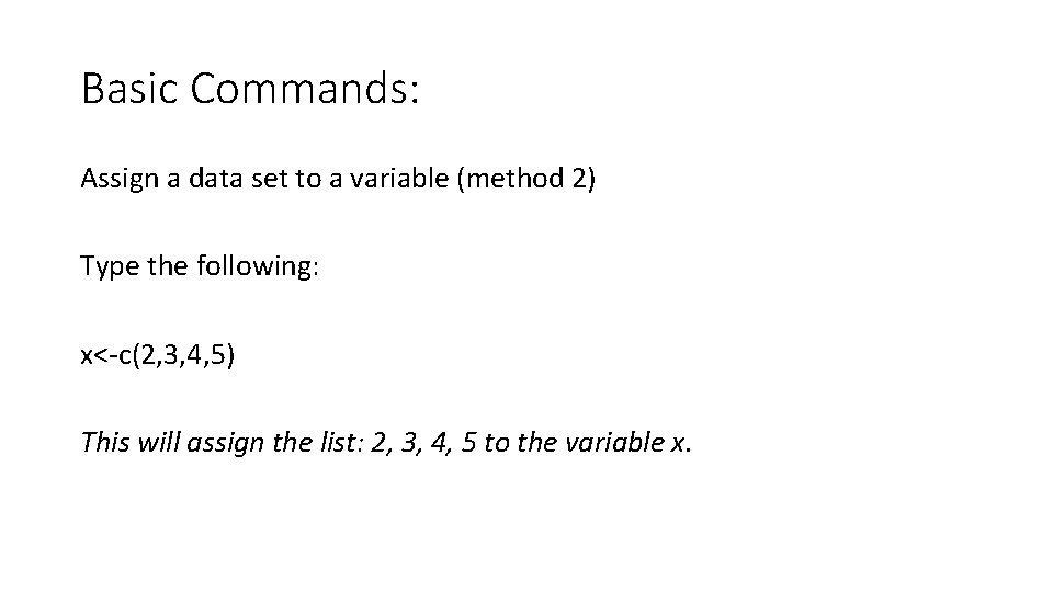
Basic Commands: Assign a data set to a variable (method 2) Type the following: x<-c(2, 3, 4, 5) This will assign the list: 2, 3, 4, 5 to the variable x.

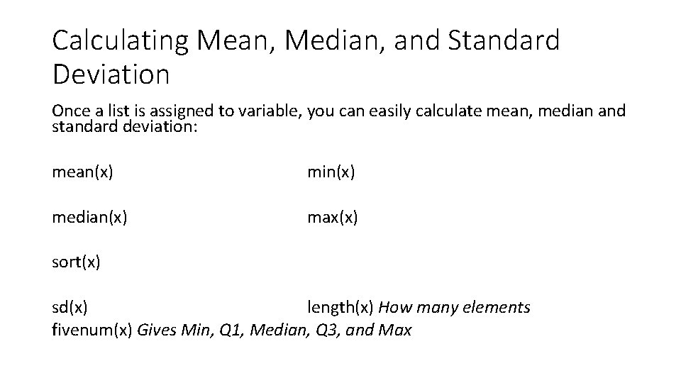
Calculating Mean, Median, and Standard Deviation Once a list is assigned to variable, you can easily calculate mean, median and standard deviation: mean(x) min(x) median(x) max(x) sort(x) sd(x) length(x) How many elements fivenum(x) Gives Min, Q 1, Median, Q 3, and Max

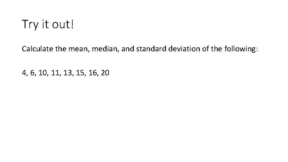
Try it out! Calculate the mean, median, and standard deviation of the following: 4, 6, 10, 11, 13, 15, 16, 20

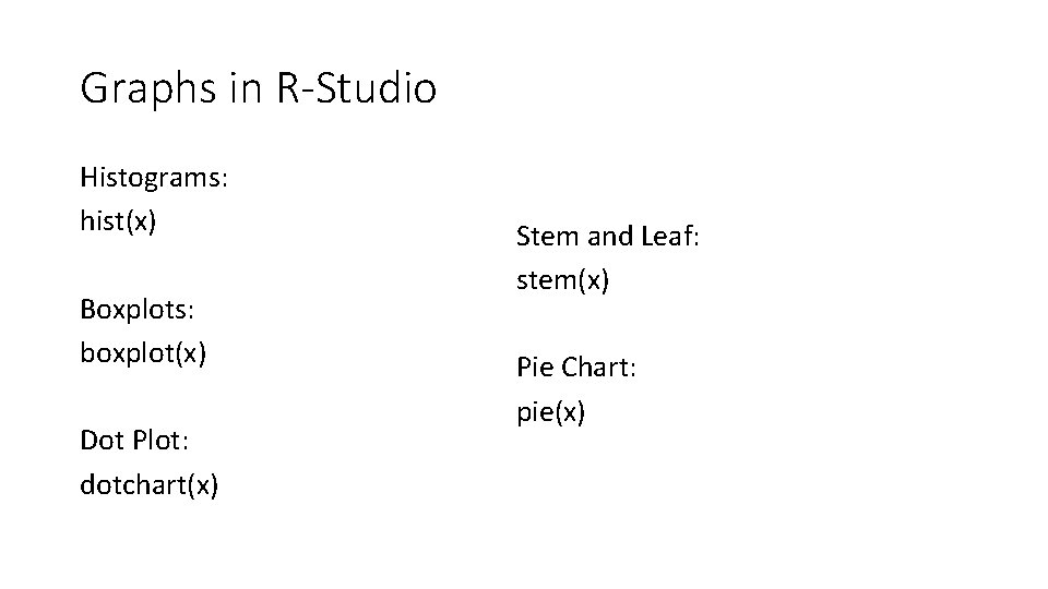
Graphs in R-Studio Histograms: hist(x) Boxplots: boxplot(x) Dot Plot: dotchart(x) Stem and Leaf: stem(x) Pie Chart: pie(x)

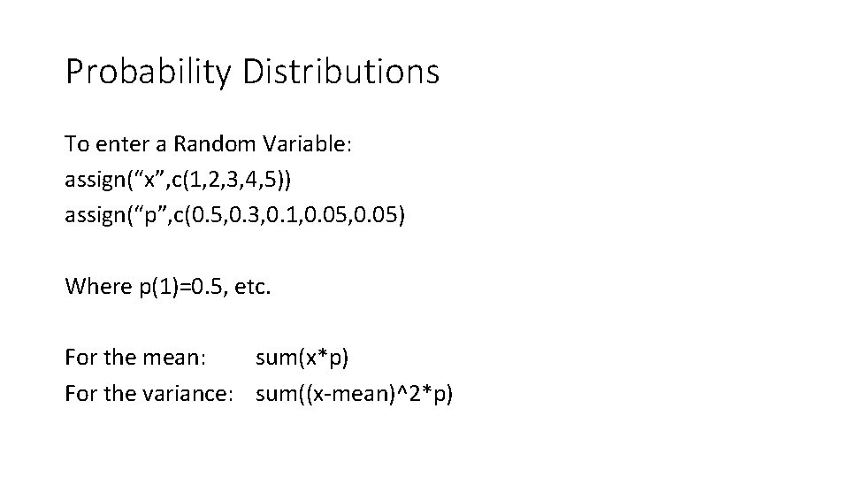
Probability Distributions To enter a Random Variable: assign(“x”, c(1, 2, 3, 4, 5)) assign(“p”, c(0. 5, 0. 3, 0. 1, 0. 05) Where p(1)=0. 5, etc. For the mean: sum(x*p) For the variance: sum((x-mean)^2*p)

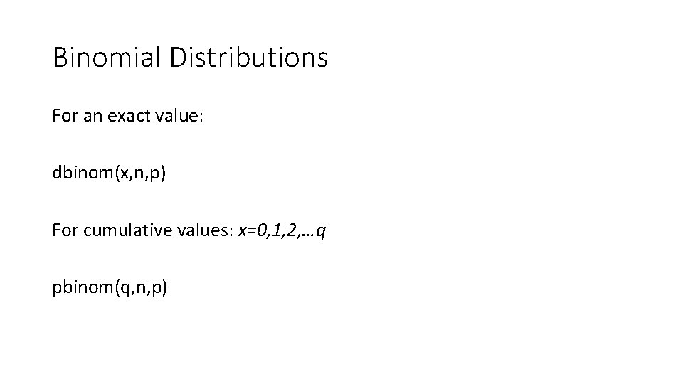
Binomial Distributions For an exact value: dbinom(x, n, p) For cumulative values: x=0, 1, 2, …q pbinom(q, n, p)

Geometric Distributions For an exact value: dgeom(n-1, p) For cumulative values: x=0, 1, 2, …q pgeom(n-1, p)

Hypergeometric Distribution For an exact value: dhyper(success, possible success, sample size, selection) For successes going from 0 through highsuccess: phyper(highsuccess, possible success, sample size, selection)

Normal Distributions: pnorm(z) will return the probability of obtaining less than a z-score of z. pnorm(x, mu, sigma) will return a probability of obtaining less than x with a mean of mu and standard deviation of sigma (standardization is not required).

Inverse Normal Distributions qnorm(p) will return the z score associated with a given probability (left tail). qnorm(p, mu, sigma) will return the x-value associated with a given probability for a mean of mu and a standard deviation of sigma (left tail).

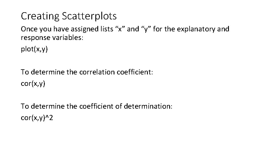
Creating Scatterplots Once you have assigned lists “x” and “y” for the explanatory and response variables: plot(x, y) To determine the correlation coefficient: cor(x, y) To determine the coefficient of determination: cor(x, y)^2

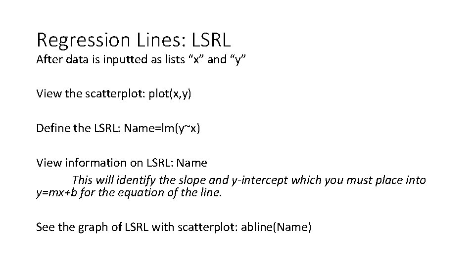
Regression Lines: LSRL After data is inputted as lists “x” and “y” View the scatterplot: plot(x, y) Define the LSRL: Name=lm(y~x) View information on LSRL: Name This will identify the slope and y-intercept which you must place into y=mx+b for the equation of the line. See the graph of LSRL with scatterplot: abline(Name)

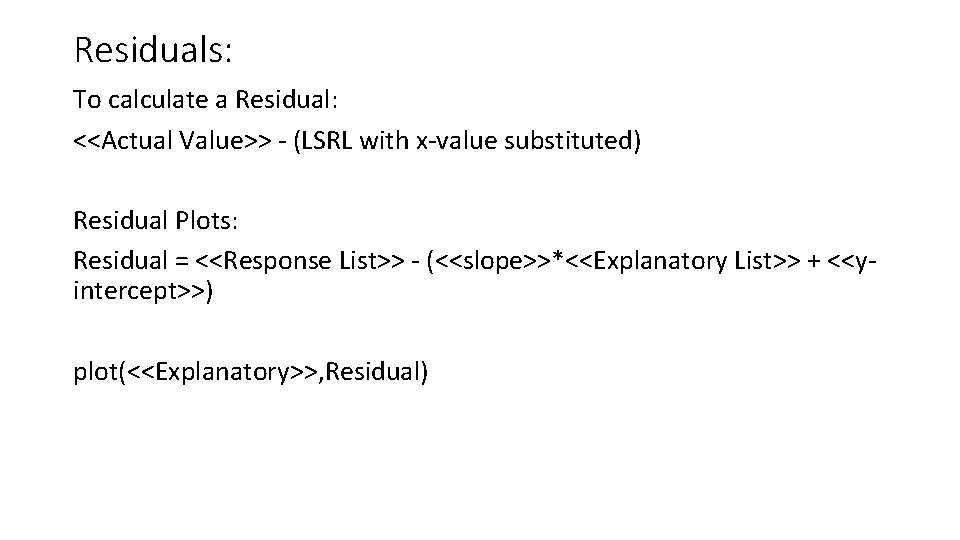
Residuals: To calculate a Residual: <<Actual Value>> - (LSRL with x-value substituted) Residual Plots: Residual = <<Response List>> - (<<slope>>*<<Explanatory List>> + <<yintercept>>) plot(<<Explanatory>>, Residual)

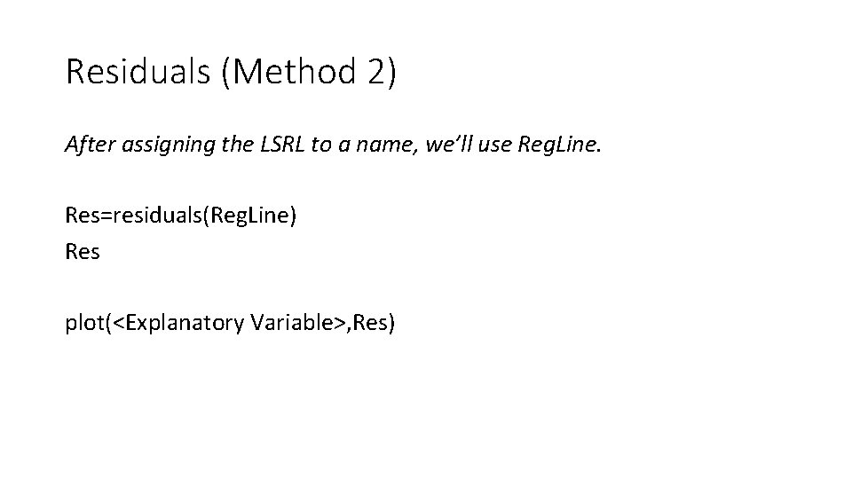
Residuals (Method 2) After assigning the LSRL to a name, we’ll use Reg. Line. Res=residuals(Reg. Line) Res plot(<Explanatory Variable>, Res)

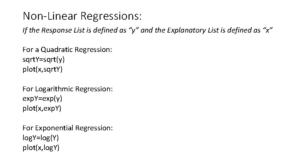
Non-Linear Regressions: If the Response List is defined as “y” and the Explanatory List is defined as “x” For a Quadratic Regression: sqrt. Y=sqrt(y) plot(x, sqrt. Y) For Logarithmic Regression: exp. Y=exp(y) plot(x, exp. Y) For Exponential Regression: log. Y=log(Y) plot(x, log. Y)

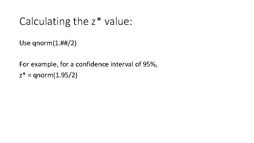
Calculating the z* value: Use qnorm(1. ##/2) For example, for a confidence interval of 95%, z* = qnorm(1. 95/2)

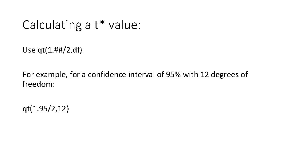
Calculating a t* value: Use qt(1. ##/2, df) For example, for a confidence interval of 95% with 12 degrees of freedom: qt(1. 95/2, 12)

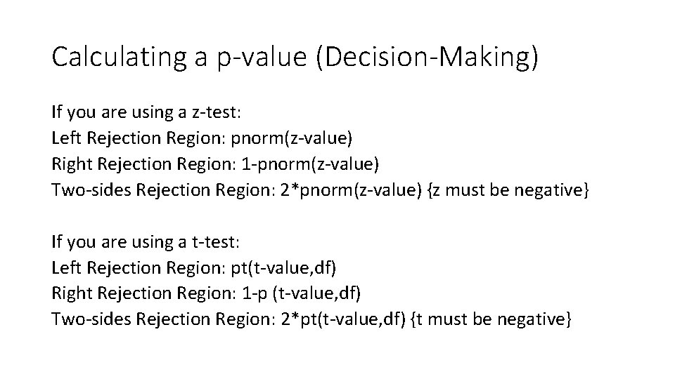
Calculating a p-value (Decision-Making) If you are using a z-test: Left Rejection Region: pnorm(z-value) Right Rejection Region: 1 -pnorm(z-value) Two-sides Rejection Region: 2*pnorm(z-value) {z must be negative} If you are using a t-test: Left Rejection Region: pt(t-value, df) Right Rejection Region: 1 -p (t-value, df) Two-sides Rejection Region: 2*pt(t-value, df) {t must be negative}

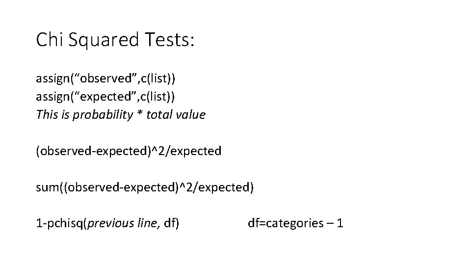
Chi Squared Tests: assign(“observed”, c(list)) assign(“expected”, c(list)) This is probability * total value (observed-expected)^2/expected sum((observed-expected)^2/expected) 1 -pchisq(previous line, df) df=categories – 1