Math 137 Hypothesis Testing The t Test Fresno

• In all of the previous examples, we assumed that we knew the

Example. The manufacturer of a new fiberglass tire claims that its average life will

Solution. H 0: The average life is at least 40, 000 miles. Ha: The

We now can compute the test statistic But there’s a catch: since we used

Since we used S instead of s, the test statistic t does NOT follow

For the sake of completeness, here’s the pdf of the Student’s t-distribution with r

Red: t distribution Blue: standard normal curve

For the t distribution with 11 df, we can compute the critical value for

Observed Significance Level 0. 002724 In Excel, the command is TDIST(3. 448, 11, 1).

Conclusion: We reject the null hypothesis. There is good reason to believe that the

Remember: If the sample is small (n < 30) and the population variance s

Example. Before a substance can be deemed safe for landfilling, its chemical properties must

Example. Certain rectangles appear more pleasing to the eye than others. The ancient Greeks

The data below shows the width-to-length ratios of beaded rectangles used by the Shoshone

Slides: 25

Download presentation

Math 137 Hypothesis Testing: The t Test Fresno State Dr. Burger

• In all of the previous examples, we assumed that we knew the population standard deviation s. • In practice, this is an extremely rare situation! • Instead, the sample standard deviation S is used in lieu of s. • This approximation is called the bootstrap estimate.

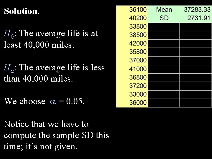
Example. The manufacturer of a new fiberglass tire claims that its average life will be at least 40, 000 miles. To verify this claim, a sample of 12 tires is tested, and the lifetimes were found to be 36, 100 42, 000 36, 800 40, 200 35, 800 37, 200 33, 800 37, 000 33, 000 38, 500 41, 000 36, 000 Test the manufacture’s claim using a = 0. 05.

Solution. H 0: The average life is at least 40, 000 miles. Ha: The average life is less than 40, 000 miles. We choose a = 0. 05. Notice that we have to compute the sample SD this time; it’s not given.

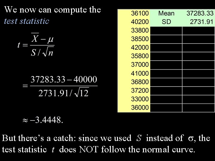
We now can compute the test statistic But there’s a catch: since we used S instead of s, the test statistic t does NOT follow the normal curve.

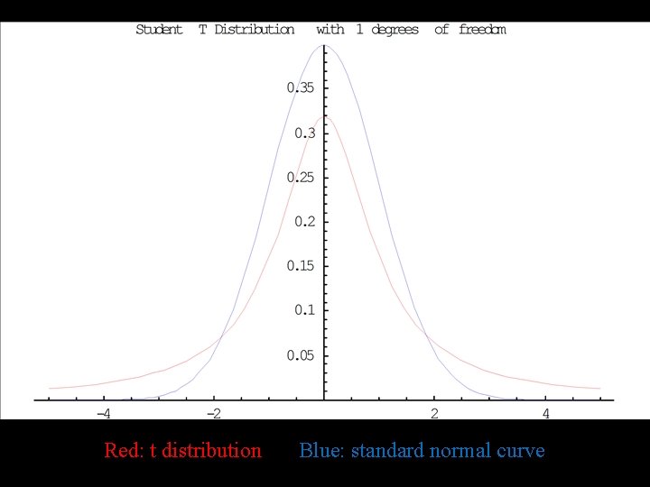
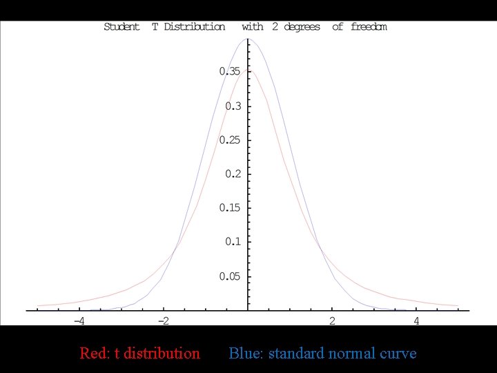
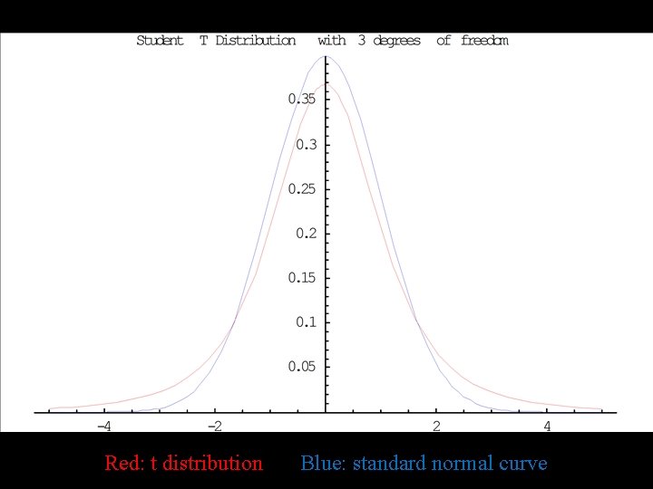
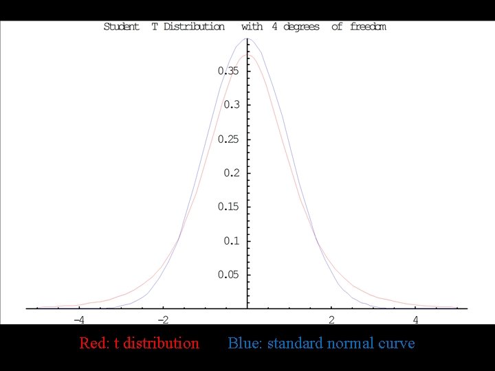
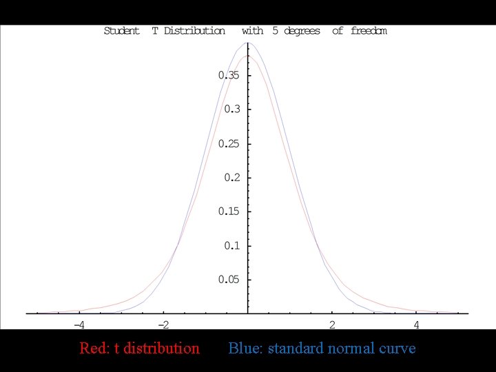
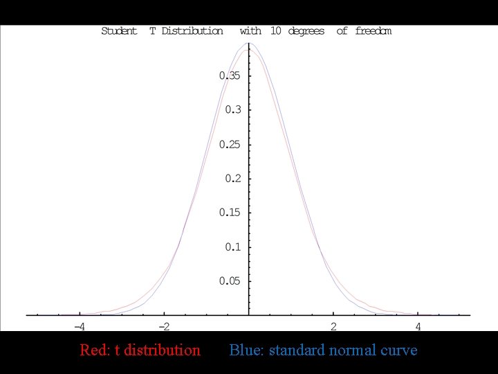
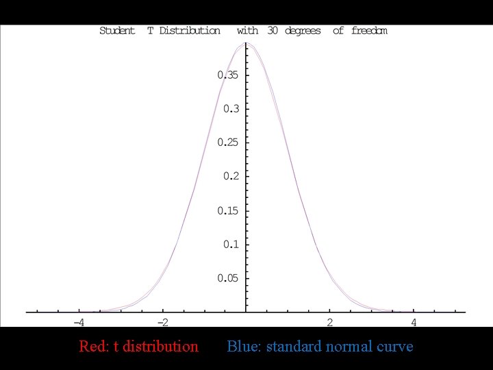
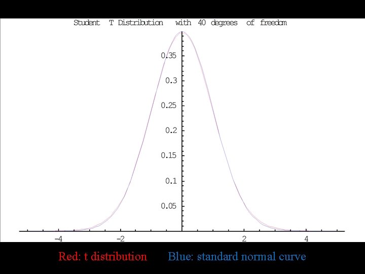
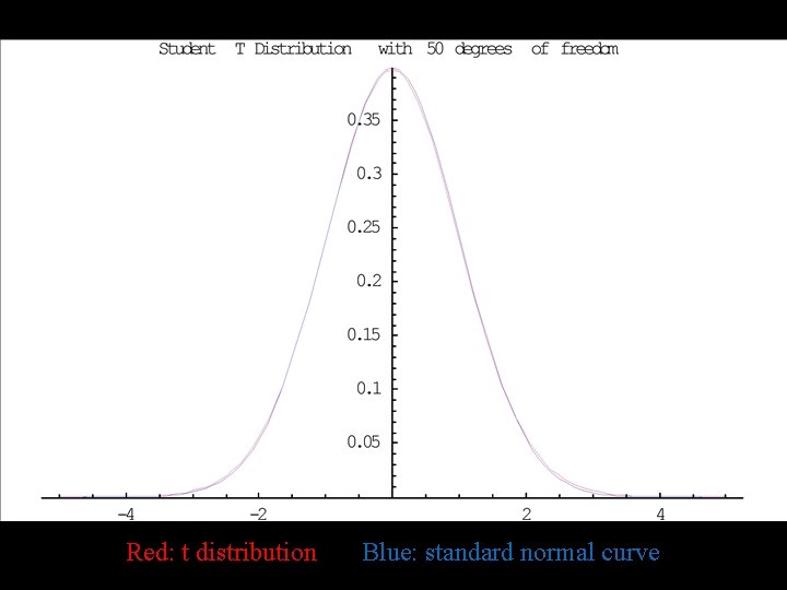
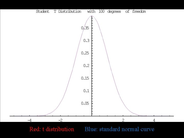
Since we used S instead of s, the test statistic t does NOT follow the normal curve. For the current problem, instead of using the normal curve to compute the observed significance level, we will use the Student t distribution with 11 degrees of freedom.

For the sake of completeness, here’s the pdf of the Student’s t-distribution with r degrees of freedom: If you find this intimidating, don’t worry: we will never use it.

Red: t distribution Blue: standard normal curve

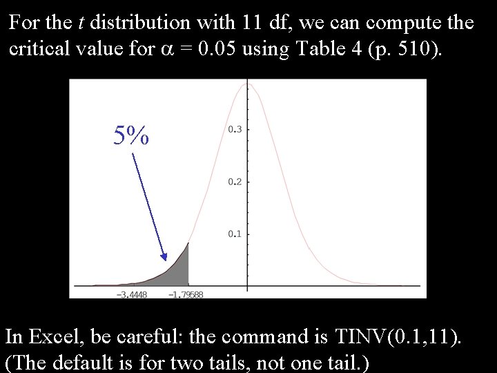
For the t distribution with 11 df, we can compute the critical value for a = 0. 05 using Table 4 (p. 510). 5% In Excel, be careful: the command is TINV(0. 1, 11). (The default is for two tails, not one tail. )

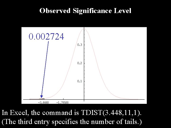
Observed Significance Level 0. 002724 In Excel, the command is TDIST(3. 448, 11, 1). (The third entry specifies the number of tails. )

Conclusion: We reject the null hypothesis. There is good reason to believe that the average lifespan of the tires is less than 40, 000 miles. Note: It is possible to compute power with the Student’s t-distribution, but the computations are much, much more complicated than the normal case (Larsen & Marx, 3 rd ed. , p. 447). Many statistical software packages are able to compute power for the t-test automatically.

Remember: If the sample is small (n < 30) and the population variance s is unknown, then we use the t-test and not the z-test. On the other hand, if either s is known or the sample is sufficiently large (n > 30), then we may safely use the z-test instead. Also, we must be careful about stating the null and alternative hypotheses so that we correctly choose whether to use a left-tail, a right-tail, or both tails.

Example. Before a substance can be deemed safe for landfilling, its chemical properties must be assessed. In a sample of six replicates of sludge from a New Hampshire wastewater treatment plant, the mean p. H was 6. 68 with a standard deviation of 0. 20. Can we conclude than the mean p. H is less than 7. 0? J. Benoit, T. Eighmy and B. Crannell, Journal of Geotechnical and Geoenvironmental Engineering 1999, pp. 877 --888.

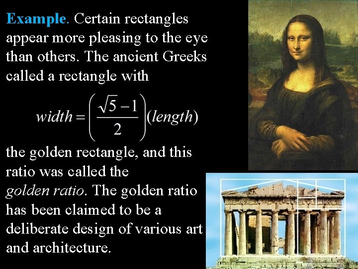
Example. Certain rectangles appear more pleasing to the eye than others. The ancient Greeks called a rectangle with the golden rectangle, and this ratio was called the golden ratio. The golden ratio has been claimed to be a deliberate design of various art and architecture.

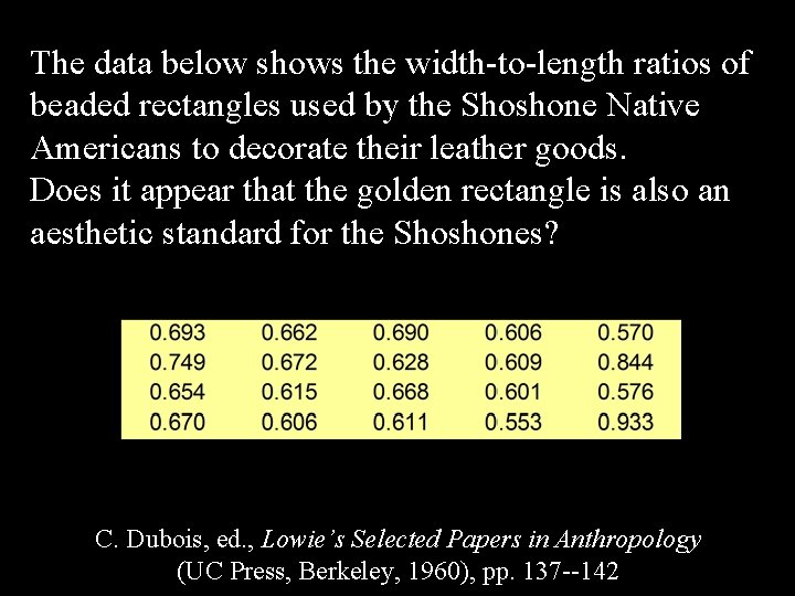
The data below shows the width-to-length ratios of beaded rectangles used by the Shoshone Native Americans to decorate their leather goods. Does it appear that the golden rectangle is also an aesthetic standard for the Shoshones? C. Dubois, ed. , Lowie’s Selected Papers in Anthropology (UC Press, Berkeley, 1960), pp. 137 --142