Materials Thermodynamic modelling Calculations of phase diagrams using

Materials Thermodynamic modelling Calculations of phase diagrams using Thermo-Calc software package Content 1. Equilibrium condition 2. Gibbs energy for elements and stoichiometric phases 3. Gibbs energy for solution phase: substitutional regular solution 4. Model for ideal gas 5. Sublattice model Interstitials, Wagner-Schottky model, ionic crystalline phases, Order/Disorder 6. Associate solution model 7. Quasichemical model 8. Two-sublattice partially ionic liquid 9. Optimisation

The Gibbs for a system and for a phase Equilibrium is minimum of the Gibbs energy of system x. B 1+3+5: G 135=n 1 G 1+n 3 G 3+n 5 G 5 1+2+4: G 124=n 1 G 1+n 2 G 2+n 4 G 4 1+3+4: G 134=n 1 G 1+n 3 G 3+n 4 G 4 2+4+5: G 245=n 2 G 2+n 4 G 4+n 5 G 5 2+4+6: G 246=n 2 G 2+n 4 G 4+n 6 G 6 2+3+5: G 235=n 2 G 2+n 3 G 3+n 5 G 5 3+4+6: G 346=n 3 G 3+n 4 G 4+n 6 G 6 3+5+6: G 356=n 3 G 3+n 5 G 5+n 6 G 6 x. A

Another approach: condition for equilibrium is equality of chemical potentials Chemical potential is partial derivative of the Gibbs energy where Ni is number of moles of component i. T, P and Nj (j≠i) For equilibrium between three phases s, r and t equilibrium condition can be written as:

Stable equilibrium, metastable equilibrium, diffusionless transformation g b a+b is stable equilibrium (global minimum of G) g+b is metastastable equilibrium (local minimum of G) a Diffusionless transformation occurs when Ga=Gb (T 0 -line) T 0 Xgg=b X Xaa=b b g=b Xba=b T 0 a+b b-equil a-equil. X aeq Xbeq Xa, Xb non-equilibrium

The Gibbs energy for elements and stoichiometric compounds FUNCTION GCORUND 298. 15 -1707351. 3+448. 021092*T-67. 4804*T*LN(T) -0. 06747*T**2+1. 4205433 E-05*T**3+938780*T**(-1); 600 Y -1724886. 06+754. 856573*T-116. 258*T*LN(T)-0. 0072257*T**2 +2. 78532 E-07*T**3+2120700*T**(-1); 1500 Y -1772163. 19+1053. 4548*T-156. 058*T*LN(T)+0. 00709105*T**2 -6. 29402 E-07*T**3+12366650*T**(-1); 3000 N !

The Gibbs energy for stoichiometric compounds The Gibbs energy of phase with constant composition at temperature T is expressed by GT = HT - ST ∙T, where HT and ST are enthalpy and entropy at temperature T. The enthalpy and entropy at temperature T are expressed by equations: where DH 0 f, el 298 is enthalpy of formation from elements, S 0298 standard entropy and CP is heat capacity, which also depends on temperature: CP= A+B∙T+C/T 2 (Maier – Kelly equation) As a result of integration of CP expressed by Maier - Kelly equation a = DH 0 f 298 -298∙A -0. 5∙ 2982∙B +298 -1∙C b = -S 0298 +A +A∙ln 298 +298∙B -0. 5∙ 298 -2∙C c= -A, d = -0. 5∙B, f = -0. 5∙C in the resulting expression of the Gibbs energy of phase

Neumann-Kopp rule is used when heat capacity data are not available. is the Gibbs energy of phase , Gi(T) is the Gibbs energy of pure element i, bi is stoichiometric coefficient This assumption means that the heat capacity of formation of the compound from elements is equal to zero: Pure oxides can be selected as components to calculate CP for mixed oxide compounds or other oxide species i. e. Mg. Si. O 3 and Ca. Si. O 3 to calculate heat capacity of diopside Ca. Mg. Si 2 O 6 Fe 2 Al 5: CP comparison of experimental data with DFT (ab-initio) and Neumann-Kopp calculations Disadvantage of using Neumann-Kopp rule is that transformations occurring in the components will be seen on CP curves as kinks at temperatures of transformations which does not have physical reason

Magnetic contribution For element or compound having magnetic ordering GHSER is referred to paramagnetic state and additional term accounting magnetic contribution is included where β is average magnetic moment, t=T/TC, where TC is critical temperature i. e Curie or Neel temperature Pressure contribution Murnaghan equation of state for solid phases where KT is isothermal bulk modulus (KT is inverse compressibility ) K’p is pressure derivative of bulk modulus The molar volume at 1 atm is expressed as function of temperature Volumetric thermal expansion is expressed as function of temperature

Equation of state for gas Ideal gas PVm=RT P 0 -1 bar Real gas Equation of Van-der-Waals Valid above critical point, for gas at low P and liquid, not valid in two phase region Vm – molar volume, P- pressure, a and b coefficients a - correction for intermolecular forces, b – for finite molecular size f – fugacity, f 0 – reference at 1 bar

The Gibbs energy for a solution phase

Lattice stability To calculate G of solution phase the Gibbs energies for both end-members A and B and mixing parameters L (0 LA, B, 1 LA, B, 2 LA, B …) should be known For liquid phase the Gibbs energies for both end-members are usually known: 0 GL and 0 GL A B For continuous solid solutions they are also known Cu-Ni fcc solid solution 0 Gfcc. Cu and 0 Gfcc. Ni For limited solid solutions G is known only for one end -member, for example, fcc solid solution in the Al-Si system: maximal solubility of Si in fcc is 1. 5 at%. How to find 0 Gfcc. Si? For compound with homogeneity range the Gibbs for both end-members is not known, for example, Ti. N fcc. How to find 0 Gfcc. Ti and 0 Gfcc. N? The Gibbs energy of metastable end member is called lattice stability. If B has different structure than A then GB with the structure of A is equal to the Gibbs energy of B in its stable state plus DG of transformation into metastable state www. sgte. orgsgte. net Unary database: collection of G(T) for all elements in stable and metastable structures

Example: thermodnamic description of Liquid phase in THERMO-CALC format for the Al-Si system FUNCTION GALLIQ 298. 15 +3028. 879+125. 251171*T-24. 3671976*T*LN(T) -0. 001884662*T**2 -8. 77664 E-07*T**3+74092*T**(-1)+7. 9337 E-20*T**7; 700 Y -271. 21+211. 206579*T-38. 5844296*T*LN(T)+. 018531982*T**2 -5. 764227 E-06*T**3+74092*T**(-1)+7. 9337 E-20*T**7; 933. 47 Y -795. 996+177. 430178*T-31. 748192*T*LN(T); 2900 N ! FUNCTION GSILIQ 298. 15 +42533. 751+107. 13742*T-22. 8317533*T*LN(T) -0. 001912904*T**2 -3. 552 E-09*T**3+176667*T**(-1)+2. 09307 E-21*T**7; 1687 Y +40370. 523+137. 722298*T-27. 196*T*LN(T); 3600 N ! PHASE LIQUID % 1 1. 0 ! CONSTITUENT LIQUID : AL, SI : ! PARAMETER G(LIQUID, AL; 0) 2. 98140 E+02 +GALLIQ#; 2900 N 91 Din ! PARAMETER G(LIQUID, SI; 0) 2. 98140 E+02 +GSILIQ#; 3600 N 91 Din ! PARAMETER L(LIQUID, AL, SI; 0) 2. 98150 E+02 -11340. 1 -1. 23394*T; 6000 N 97 Feu ! PARAMETER L(LIQUID, AL, SI; 1) 2. 98150 E+02 -3530. 93+1. 35993*T; 6000 N 97 Feu ! PARAMETER L(LIQUID, AL, SI; 2) 2. 98150 E+02 2265. 39; 6000 N 97 Feu !

Redlich-Kister parameters The contribution to the enthalpy of mixing for the first five terms (0 L-4 L) for the same value of the parameter equal to 20000 J/mol in the Redlich-Kister power series Parameters n. Lij can depend on temperature n. Lij=naij+nbij. T

Non-ideal behavior Eij Eii Ejj Energy difference eij for bonds between unlike atoms Eij and similar atoms Eii and Ejj eij=Eij-0. 5(Eii+Ejj) eij<0 tendency for unlike atoms to be together, forming compounds eij>0 Tendency to phase separation, forming of miscibility gaps For substitutional regular solution model z - number of bonds

Application of substitutional model Substitutional model is used to describe : v liquid phase in metallic systems v Solid metallic phase if atoms are mixing in one single sublattice, the second being empty: i. e. fcc (Fe, Ni)1(Va)1, bcc (Fe, Ni)1(Va)3

Example: Al-Bi system a. – calculated phase diagram of Al-Bi system b. – calculated integral properties at 1400 K c. – calculated activities at 1400 K

Example Al-Y system a. – calculated phase diagram for Al-Y system b. – calculated integral properties of liquid at 1800 K c. - calculated activity of Al and Y in liquid at 1800 K.

Ternary interaction parameters n=3 The excess energy consists from binary interactions (Muggianu extrapolation) Muggianu (1975) For ternary system binary excess contribution is: bin, EG m=x 1 x 2{ 0 L 12+ 1 L 12(x 1 -x 2)}+x 1 x 3{ 0 L 13+ 1 L(x bin, EG 1 -x 3)}+x 2 x 3{ Ternary excess contribution tern, EGm=x 1 x 2 x 3 L 123=x 11 L 123+x 22 L 123+x 33 L 123 For multicomponent system m=x 1 x 2 L 12+x 1 x 3 L 13+x 2 x 3 L 23 0 L 23+ 1 L 23(x 2 -x 3)}

Other methods of extrapolation into ternary system Kohler Geometric presentation: Kohler and Muggianu models are symmetric, Toop is asymmetric Kohler model assumes that xi/(xi+xj)=const Toop model assumes that x 1=const The difference between models exists only L has higher order parameters L 1, L 2 … (b) Toop Model [1965 Too]

Model for multicomponent ideal gas Gas phase usually consists of many constituents (species) which mixed ideally where 0 Gi – the Gibbs energy of constituent i, yi – its fraction The Gibbs energy of gas phase depends on pressure where bij is stoichiometric coefficient of gas constituent, p 0 – atmospheric pressure, yi=pi/p constitutent fraction equal to ratio of partial pressure pi to total pressure p V=n. RTp-1 equation of state for ideal gas

Example: system H-O Gas constituents H 2, O 2, H 2 O, O, H, O 3 There additional internal degrees of freedom, because constituents can react with each other T 5 T 4 T 3 T 2 2 H 2+O 2=2 H 2 O, 2 H=H 2, 2 O=O 2 etc T 1<T 2<T 3<T 4<T 5

Sublattice model Fluorite Structure 2 -sublattice model (Zr+4, Y+3)1(O-2, Va)2 A 2/B 2 ordering A 2: (Fe, Al)1(Va, C)3 Second sublattice is interstitials B 2: (Fe, Al)0. 5(Va, C)3 First sublattice is divided into two for B 2 model and the third sublattice is interstitials

Sublattice Model (A, B)a(C, D)c The Gibbs energy of a phase consists from Reference Surface Energy, Configurational Entropy and Excess Energy terms Reference surface energy is expressed as 0 G is the Gibbs energy of formation of compound iajc, also called end-member, y’i and y’’ j are mole fraction of species i and j in the first and second sublattice Configurational entropy is expressed as ij

Sublattice model For considered case (A, B)a(C, D)c: The excess energy contribution is described as regular solution on each sublattice L – are Redlich-Kister series The end members are related with each others by Reciprocal Reaction: Aa. Dc+Ba. Cc=Aa. Cc+Ba. Dc

Example: modelling of Laves phases in Cr-Ti system Laves phase modelling: a-Ti. Cr 2 C 15, b-Ti. Cr 2 C 36, g-Ti. Cr 2 C 14 (Cr, Ti)2(Ti, Cr)1 Cr 2 Ti, Cr 2 Cr, Ti 2 Ti, Ti 2 Cr a-Ti. Cr 2 - C 15 CN 12 16 d Cr CN 16 8 a Ti Mixing parameters Cr 2 Ti+Ti 2 Cr=Cr 2 Cr+Ti 2 Ti DGrec=0

Phase diagram of the Cr-Ti system b-Bcc (Cr, Ti)1(Va)3 a-Hcp (Ti, Cr)1(Va)0. 5 a-Ti. Cr 2, b-Ti. Cr 2, g-Ti. Cr 2 (Cr, Ti)2(Ti, Cr)1 Liquid (Cr, Ti)

Sublattice model to describe interstitials Common application of Sublattice model is to describe interstitial solution of C, N, O and other non-metals in metallic phases FCC_A 1 (Fe, Cr, Ni)1(Va, C, N, O, B)1 Some carbides and nitrides also forms fcc structure and can be described as single phase which forms a miscibility gap. Example: Fe-N system Liquid (Fe, N)1 Fcc_A 1 (Fe)1(Va, N)1 Bcc_A 2 (Fe)1(Va, N)3 Hcp_A 3 (Fe)2(Va, N)1 Fe 4 N - stoichiometric

Wagner-Schottky model to describe defects Wagner-Schottky model is to describe narrow homogeneity range in compounds due to various type of defects (A, X)a(B, Y)b Aa. Bb is ideal compounds, X and Y are defects. Defects can be: 1) anti-site atoms, B in sublattice for A and A in sublattice for B (A, B)a(B, A)b 2) Vacancies (A, B)a(B, Va)b 3) Interstitials (A)a(B)b(Va, A, B)c (A, X)a(B, Y)b Wagner-Schottky model consider one defect for each sublattice and contains three parameters 0 GA: B, D 0 GX: B and D 0 GA: Y (energy of formation of compound, energy of formation of defect on the first and second sublattices). Wagner. Schottky model is applicable when fraction of defects is very small and defects are non-interacting

Wagner-Schottky model – relations with sublattice model (A, X)a(B, Y)b 0 G Aa. Bb, D 0 GA: Y, D 0 GX: B are parameters of Wagner-Schottky model n. X is number of X in A sites, n. Y number of Y in B sites, n is total number of sites Example: Y-O system Y 2 O 3_R and Y 2 O 3_H are modelled by Wagner-Schottky model (Y+3)2(O-2, Va)3

Ionic crystalline phases Example: Fe-O system, modelling of wüstite Fex. O phase Fex. O: (Fe+2, Fe+3, Va)1(O-2)1 Electroneutrality condition: 2 Fe+3 O-2+Va. O-2=Fe 2 O 3 Crystal structure of wüstite

Modelling of Spinel in the Mg. O-Al 2 O 3 system Spinel Mg 1 Al 2 O 4 (Mg+2, Al+3)T 1(Al+3, Mg+2)O 2(Va)I 2 O 4 (Mg+2, Al+3)T 1(Al+3, Mg+2, Va)O 2(Mg+2, Va)I 2 O 4 Hallstedt, 1992

Modelling of Spinel phase (Mg+2, Al+3)T 1(Al+3, Mg+2)O 2(Va)I 2 O 4 Al. Al 2 O 4+1+Al. Mg 2 O 4 -1=2 Mg. Al 2 O 4 (Mg+2, Al+3)T 1(Al+3, Mg+2, Va)O 2(Va)I 2 O 4 Al. Va 2 O 4 -5+5 Al. Al 2 O 4+1=8 g-Al 2 O 3

Modelling of Spinel phase (Mg+2, Al+3)T 1(Al+3, Mg+2)O 2(Va, Mg+2)I 2 O 4 Mg. Mg 2 Va. O 4 -2+Mg. Mg 2 O 4+2=8 g-Mg. O Al. Mg 2 O 4+3+3 Al. Mg 2 Va. O 4 -1=2 Mg 5 Al 2 O 8

Thermodynamic modelling of pyrochlore structure Zr+4 La+3 (La+3, Zr+4)2(Zr+4, La+3)2(O-2, Va)6(O-2)1(Va, O-2)1

Sublattice model to describe order/disorder Al-Fe system 0 G A: B= 0 G B: A 0 G A: A= 0 Gbcc A 0 G B: B= 0 Gbcc B LA, B: A=LA, B: B=LA, B: * LA: A, B=LB: A, B=L*: A, B LA, B: *=L*: A, B

Order/Disorder In case of disorder y‘i=y“i=xi LA, B: *=L*: A, B + 0 G A= 0 G A: A 0 G B= 0 G B: B LA, B=20 GA: B-0 GA: A-0 GB: B+2 LA, B: * (y replaced by x)

Example: oder/disorder in fcc phase Au. Cu L 10 Au 3 Cu, Au. Cu 3 L 12 (Au, Cu)(Au, Cu) L 12 (Ni, Si)0. 75(Ni, Si)0. 25

Associate solution model Systems with short-range-order (SRO) Unlike atoms stay together, but attractive forces are not strong enough to form a stable chemical molecule New constituent (species) is introduced what creates additional internal degrees of freedom (A, Aa. Bb, B) The reference surface energy and configurational entropy are described where yi is constituent fraction, Gi is the Gibbs energy of constituent i. The excess energy is described the same way as in substitutional model, treating each pair of constituents as independent parameter

Example: Te-Zn system Liquid (Te, Zn) Calculated integral properties and activities at 1900 K

Example: Al-N system Liquid (Al, Al. N, N) FCC (Al)1(Va)1 - stoichiometric Al. N (Al+3)1(N-3)1 - stoichiometric Gas (Al, N, N 2, N 3)

Example of ceramic system K 2 O-Al 2 O 3 -Si. O 2 Yazhenskikh, Hack, Müller (2011) List of species in liquid K 2 O, Al 2 O 3, Si 2 O 4 2/3 K 2 Si. O 3 1/2 K 2 Si 2 O 5 1/3 K 2 Si 4 O 9 KAl. O 2 1/3 K 2 Al 4 O 7 1/4 Al 6 Si 2 O 13 1/2 KAl. Si 2 O 6 2/3 KAl. Si. O 4 List of solid phases K 2 Si. O 3, K 2 Si 2 O 5, K 2 Si 4 O 9, KAl. O 2, KAl 9 O 14, K 2 Al 12 O 19, Al 6 Si 2 O 13, KAl. Si. O 4, KAl. Si 3 O 8 (microcline, K-feldspar, sanidine), KAl. Si 2 O 6 (luecite)

Quasi-chemical model Model proposed by Guggenheim for systems with SRO (short-range-order) The formation of the bonds described by chemical reactions AA+BB=AB+BA AB and BA are different in solid phase because orientations of bonds in crystals are important z – is number of bonds per atom x. A=y. AA+0. 5(y. AB+y. BA) x. B=y. BB+0. 5(y. AB+y. BA) Mass balance Entropy is overestimated because if z=2 it is identical to entropy of gas Modified entropy In case there is no SRO: y. AA=x. A 2, y. BB=x. B 2, y. AB=y. BA=x. A∙x. B

Calculations with modified quasi-chemical model for liquid System Ag-Zr (Kang and Jung, 2010) System Mg. O-Al 2 O 3 -Si. O 2 Jung, Decterov, Pelton (2004)

The cell model M. L. Kapoor, G. M. Frohberg, H. Gaye and J. Welfringer The model was developed for oxide slag and it has a special form of quasi-chemical entropy. Different cells with one anion and two cations were considered. Cell can have two identical or two different cations. Cells mix essentially ideally, with equilibria among the cells: [Mg-O-Mg] + [Si-O-Si] = 2 [Mg-O-Si] DG° < 0 • • • Quite similar to Modified Quasichemical Model Accounts for ionic nature of slags and short-range-ordering. Has been applied with success to develop databases for multicomponent systems. ui metal stoichiometry, ni is the oxygen stoichiometry in Mu. On Di is a sum of component oxides, nj is the oxygen stoichiometry, xj is mole fraction of component oxide, i. e. cells with only one type of cations

Two-sublattice partially ionic liquid model C –cations, A –anions, n-electric charge, Va –vacancies B-neutral species The number of sites P and Q vary with composition in order to maintain electro neutrality The Gibbs energy expression for this model G=srf. Gm-Tcnf. Sm+EGm

Model parameters 0 G is the Gibbs energy of formation of (ni+nj) moles of liquid Ci. Aj, 0 G and 0 G are the Gibbs energy of liquid metal C and liquid B Ci: Aj The excess parameters Li 1, i 2: j represents interaction between two cations, e. g. in the Ca. O-Mg. O system LCa+2, Mg+2: O-2 Li 1, j 2: Va represents interaction between metals in metallic liquid , e. g. in the system Ca-Mg LCa, Mg Li: j 1, j 2 represents interaction between two anions, e. g. in the system Na. Cl-Na. NO 3 LNa+1: Cl-1, NO 3 -1 Li: j, Va is interaction between metal atom and anion, e. g. system Fe-O LFe+2: O-2, Va Li: j, k is interaction between anion and neutral species, e. g. Fe-S system LFe+2: S-2, S Li; Va, k is interaction between metal atom and neutral species, e. g. Fe-C system LFe+2: Va, C Lk 1, k 2 is interaction between two neutral species, e. g. Si 3 N 4 -Si. O 2 system LSi 3 N 4, Si. O 2

Example: Fe-O system (Fe+2)P(O-2, Va, Fe. O 1. 5)Q Example: Fe-Si-O system (Fe+2, Si+4)P(O-2, Si. O 4 -4, Va, Fe. O 1. 5, Si. O 2)Q Fe 2 O 3+Si. O 2+Fe 3 O 4 Liq 1 Liq Fe 2 Si. O 4+Fe 3 O 4 Fe. O+Fe 2 Si. O 4 Fe. O+Fe Fe+Si. O 2 Faya=Fe 2 Si. O 4 Wüs=Fe. O 1 -x Quartz, tri, cri=Si. O 2 Magnetite=Fe 3 O 4 Hematite=Fe 2 O 3

Compatibility of two sublattice partially ionic liquid model with other models Partially ionic liquid can describe metallic liquids (for this vacancies are introduced in anionic sublattice, non-metallic, polymeric liquids, e. g. liquid sulfur or Si. O 2 (for this neutral species are introduced in anionic sublattice) and ionic liquids, e. g. liquid salts like Na. Cl, Na. NO 3 (cations in the cationic sublattice and anions in the anionic sublattice) Substitutional model Two-sublattice partially ionic liquid (Fe, Cr) (Fe+2, Cr+3)P(Va)Q (Fe, C) (Fe+2)P(Va, C)Q P=Q Associate model (Cu, Cu 2 S, S) (Ca, Ca. O, Ca 2 Si. O 4, Si. O 2) (Cu+1)P(S-2, Va, S)Q (Ca+2)P(O-2, Si. O 4 -4, Va, Si. O 2)Q

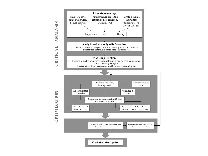
Computational Thermodynamics Estimates Theory DTA, Calorimetry, EMF, Knudsen Effusion, Metallography, X-ray Diffractometry, . . . Quantum Mechanics, Statistical Thermodynamics Optimization Experiments CALculation of PHAse Diagrams Models with adjustable Parameters Ab-initio Calculation Adjustment of Parameters www. calphad. org Thermodyn. Functions G, H, S, C p Storage in Databases Equilibrium Calculations CALPHAD Equilibria Phase Diagrams Application Graphical Representation Kinetics

Experimental data 1. Phase equilibrium data 1 a. Heat treatment to reach equilibrium, XRD for identification of phases, SEM/EDX or microprobe to determine composition of phases Conditions of equilibrium: T and phases in equilibrium = fixed Experimental results: composition of phases 1 b. Differential thermal analysis (DTA), XRD before and after DTA Condition of equilibrium: phases in equilibrium =fixed, composition of liquid is fixed=X(bulk) (liquidus), composition of solid is fixed=X(bulk) (solidus) Experimental results: temperature of solidus/liquidus F F B B B F B BB B B F B DTA: at fixed composition transformation occurs at 1500°C XRD, SEM/EDX: At 1600°C in equilibrium are phases: F (0. 58, 0. 25, 0. 17) and B (0. 81, 0. 03, 0. 16) [Sm, Zr, Y]

Phase equilibrium data Equilibration of sample with gas mixtures of known activity (CO/CO 2, H 2/H 2 O etc. ) amount of released/consumed gases are controlled gravimetrically or samples are quenched and their composition is determined by XRD, SEM/EDX and by chemical analysis Conditions: two phase fixed, T and a(O 2)=fixed Experimental data: compositions of phases Thermogravimetric analysis (TG) is method which measure change of sample mass during applied temperature-time program in a well defined atmosphere. It can be used to determine temperature of decomposition of sample accompanied by gas formation or study of reduction/oxidation reactions

2. Experimental thermodynamic data: DSC – differential scanning calorimetry – heat capacity Cp, enthalpy of transformation (also by DTA) Solution calorimetry, combustion calorimetry – enthalpy of formation from components, enthalpy of mixing Direct reaction calorimetry – enthalpy of formation of compounds Mixing isoperibolic calorimetry – partial enthalpies of mixing Adiabatic calorimetry – Cp from very low temperature up to room temperature and calculation of standard entropy S 0298 EMF- activity, chemical potentials, the Gibbs energy of formation Vapor pressure data (Knudsen effusion cell with mass-spectrometry) - activity, chemical potentials, the Gibbs energy of formation

The Zr. O 2 -YO 1. 5 system Enthalpy of mixing in Fluorite phase at 977 K Phase diagram Activity of Zr. O 2 in Fluorite phase Fluorite structure (Zr+4, Y+3)(O-2, Va)2