Mat Lab Palm Chapter 5 2 D 3

Mat. Lab – Palm Chapter 5 2 -D & 3 -D Plots Class 13. 1 Palm Chapter: 5. 1 -5. 4 & 5. 8 6/3/2021 ENGR 111 A Fall 2004 1

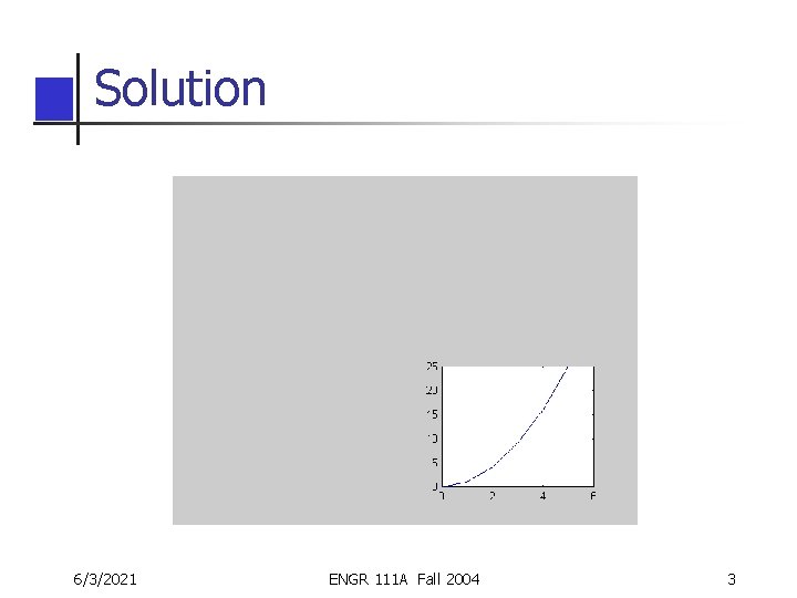
RAT 13. 1 n n n As in INDIVIDUAL you have 2 minutes to answer the following question. What is the result of the following subplot and plot commands: x = [0: 5]; y = x. ^2; subplot(2, 2, 4) plot(x, y) Answer: Creates a plot of y vs. x on a figure window with four “panes”. This plot would be in the lower, right pane of the figure window. 6/3/2021 ENGR 111 A Fall 2004 2

Solution 6/3/2021 ENGR 111 A Fall 2004 3

Learning Objectives for Today’s Class n Students should be able to: n n n 6/3/2021 Use the 2 -D (X-Y) Plotting Functions. Make Subplots and Overlay Plots. Use Special Plot Functions. Use the Plot Editor. Use the 3 -D (X-Y-Z) Plot Functions. ENGR 111 A Fall 2004 4

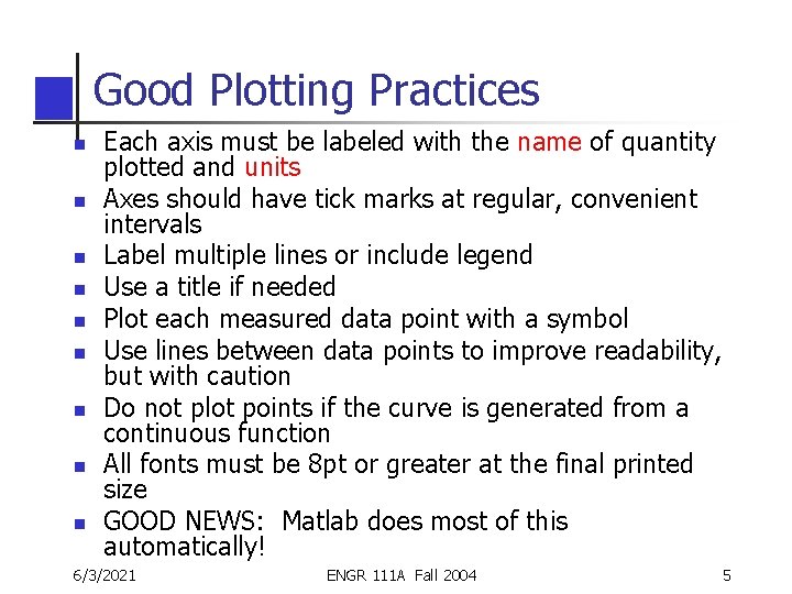
Good Plotting Practices n n n n n Each axis must be labeled with the name of quantity plotted and units Axes should have tick marks at regular, convenient intervals Label multiple lines or include legend Use a title if needed Plot each measured data point with a symbol Use lines between data points to improve readability, but with caution Do not plot points if the curve is generated from a continuous function All fonts must be 8 pt or greater at the final printed size GOOD NEWS: Matlab does most of this automatically! 6/3/2021 ENGR 111 A Fall 2004 5

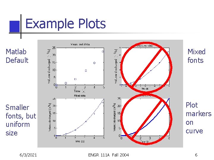
Example Plots Matlab Default Mixed fonts Smaller fonts, but uniform size Plot markers on curve 6/3/2021 ENGR 111 A Fall 2004 6

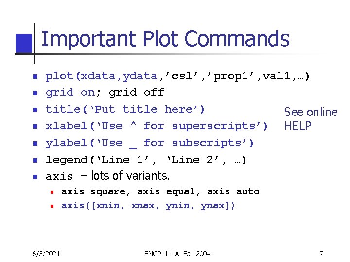
Important Plot Commands n n n n plot(xdata, ydata, ’csl’, ’prop 1’, val 1, …) grid on; grid off title(‘Put title here’) See online xlabel(‘Use ^ for superscripts’) HELP ylabel(‘Use _ for subscripts’) legend(‘Line 1’, ‘Line 2’, …) axis – lots of variants. n n 6/3/2021 axis square, axis equal, axis auto axis([xmin, xmax, ymin, ymax]) ENGR 111 A Fall 2004 7

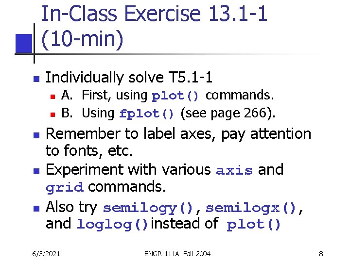
In-Class Exercise 13. 1 -1 (10 -min) n Individually solve T 5. 1 -1 n n n A. First, using plot() commands. B. Using fplot() (see page 266). Remember to label axes, pay attention to fonts, etc. Experiment with various axis and grid commands. Also try semilogy(), semilogx(), and loglog()instead of plot() 6/3/2021 ENGR 111 A Fall 2004 8

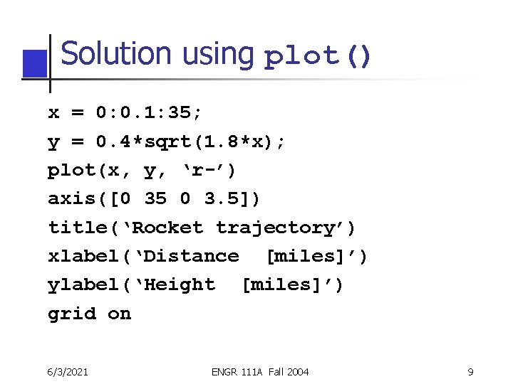
Solution using plot() x = 0: 0. 1: 35; y = 0. 4*sqrt(1. 8*x); plot(x, y, ‘r-’) axis([0 35 0 3. 5]) title(‘Rocket trajectory’) xlabel(‘Distance [miles]’) ylabel(‘Height [miles]’) grid on 6/3/2021 ENGR 111 A Fall 2004 9

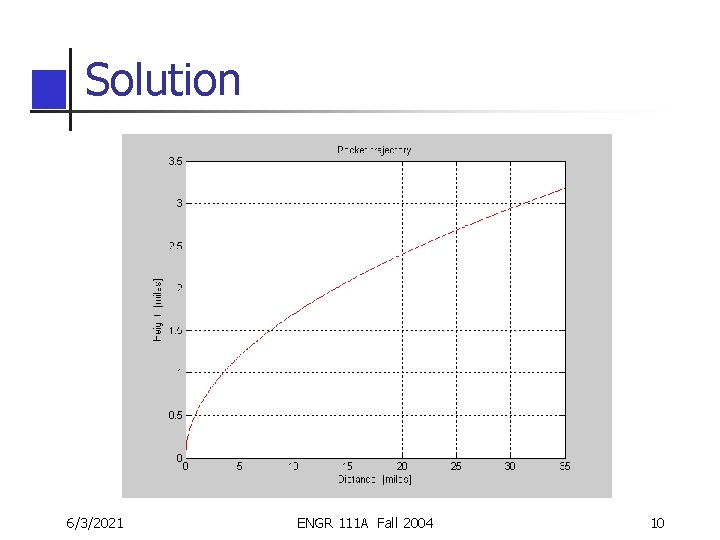
Solution 6/3/2021 ENGR 111 A Fall 2004 10

Solution using fplot() f = ‘ 0. 4 * sqrt(1. 8*x)’ fplot(f, [0 35]) axis([0 35 0 3. 5]) title(‘Rocket trajectory’) xlabel(‘Distance [miles]’) ylabel(‘Height [miles]’) grid on 6/3/2021 ENGR 111 A Fall 2004 11

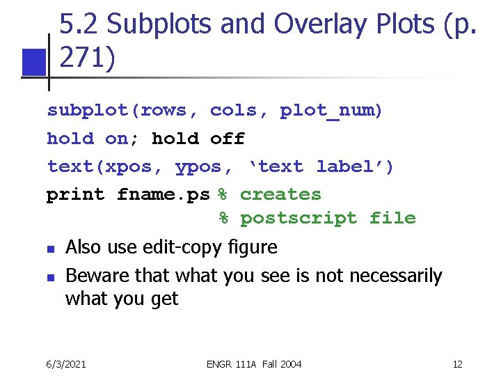
5. 2 Subplots and Overlay Plots (p. 271) subplot(rows, cols, plot_num) hold on; hold off text(xpos, ypos, ‘text label’) print fname. ps % creates % postscript file n n Also use edit-copy figure Beware that what you see is not necessarily what you get 6/3/2021 ENGR 111 A Fall 2004 12

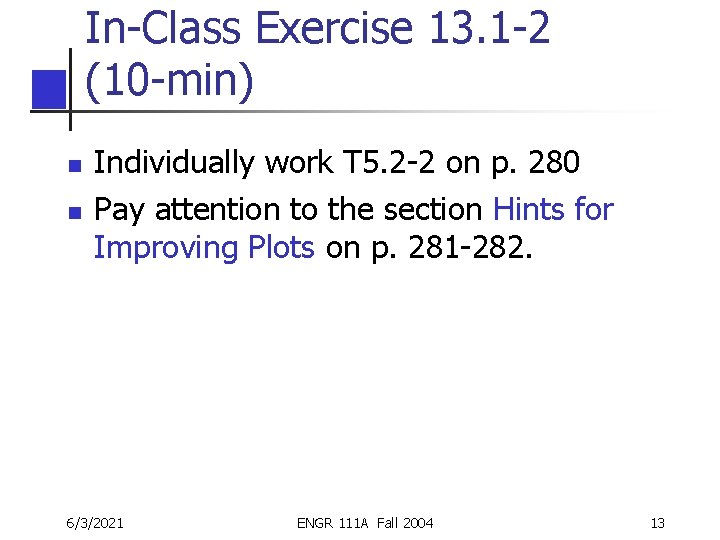
In-Class Exercise 13. 1 -2 (10 -min) n n Individually work T 5. 2 -2 on p. 280 Pay attention to the section Hints for Improving Plots on p. 281 -282. 6/3/2021 ENGR 111 A Fall 2004 13

Solution x = [0 1 2 3 4 5]; y 1 = [11 13 8 7 5 9]; y 2 = [2 4 5 3 2 4]; plot(x, y 1, 'ko-') hold on plot(x, y 2, 'kd--') legend('Data set 1', 'Data set 2') xlabel('Independent variable [--]') ylabel('Dependent variable [--]') 6/3/2021 ENGR 111 A Fall 2004 14

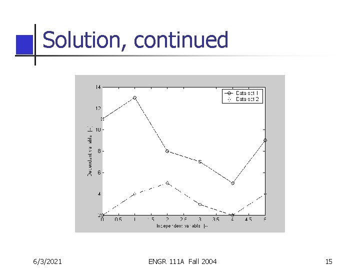
Solution, continued 6/3/2021 ENGR 111 A Fall 2004 15

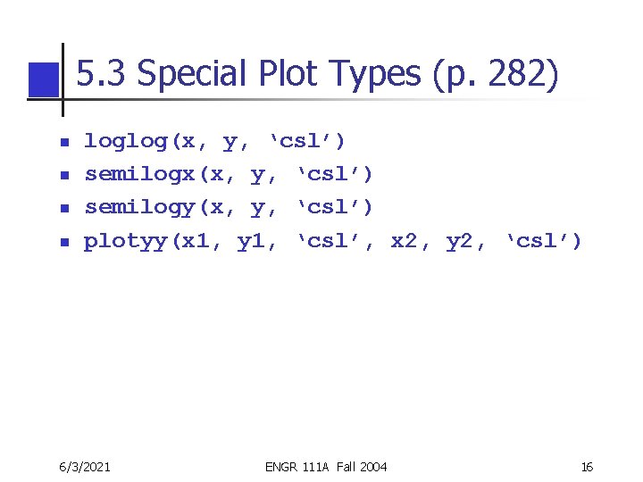
5. 3 Special Plot Types (p. 282) n n loglog(x, y, ‘csl’) semilogx(x, y, ‘csl’) semilogy(x, y, ‘csl’) plotyy(x 1, y 1, ‘csl’, x 2, y 2, ‘csl’) 6/3/2021 ENGR 111 A Fall 2004 16

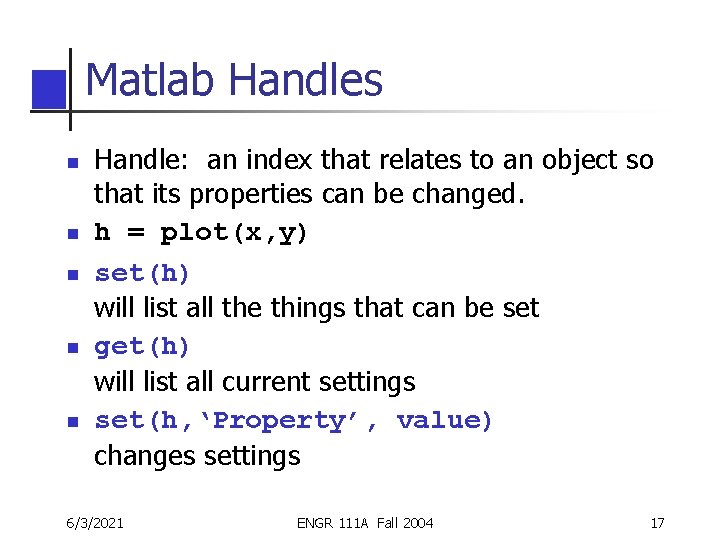
Matlab Handles n n n Handle: an index that relates to an object so that its properties can be changed. h = plot(x, y) set(h) will list all the things that can be set get(h) will list all current settings set(h, ‘Property’, value) changes settings 6/3/2021 ENGR 111 A Fall 2004 17

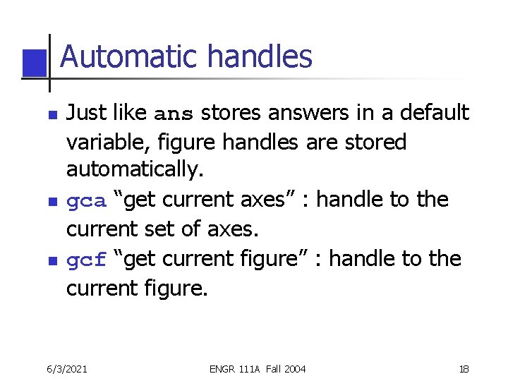
Automatic handles n n n Just like ans stores answers in a default variable, figure handles are stored automatically. gca “get current axes” : handle to the current set of axes. gcf “get current figure” : handle to the current figure. 6/3/2021 ENGR 111 A Fall 2004 18

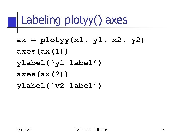
Labeling plotyy() axes ax = plotyy(x 1, y 1, x 2, y 2) axes(ax(1)) ylabel(‘y 1 label’) axes(ax(2)) ylabel(‘y 2 label’) 6/3/2021 ENGR 111 A Fall 2004 19

In-Class Exercise 13. 1 -3 (10 -min) n n Individually solve T 5. 3 -1 on p. 291 You may learn how to use the Plot Editor (section 5. 4) on your own to edit your plots. 6/3/2021 ENGR 111 A Fall 2004 20

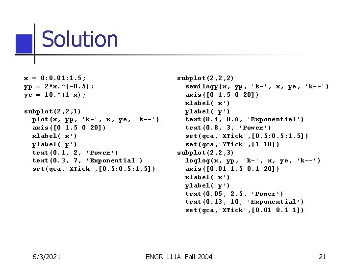
Solution x = 0: 0. 01: 1. 5; yp = 2*x. ^(-0. 5); ye = 10. ^(1 -x); subplot(2, 2, 1) plot(x, yp, 'k-', x, ye, 'k--') axis([0 1. 5 0 20]) xlabel('x') ylabel('y') text(0. 1, 2, 'Power') text(0. 3, 7, 'Exponential') set(gca, 'XTick', [0. 5: 1. 5]) 6/3/2021 subplot(2, 2, 2) semilogy(x, yp, 'k-', x, ye, 'k--') axis([0 1. 5 0 20]) xlabel('x') ylabel('y') text(0. 4, 0. 6, 'Exponential') text(0. 8, 3, 'Power') set(gca, 'XTick', [0. 5: 1. 5]) set(gca, 'YTick', [1 10]) subplot(2, 2, 3) loglog(x, yp, 'k-', x, ye, 'k--') axis([0. 01 1. 5 0. 1 20]) xlabel('x') ylabel('y') text(0. 05, 2. 5, 'Power') text(0. 13, 10, 'Exponential') set(gca, 'XTick', [0. 01 0. 1 1]) ENGR 111 A Fall 2004 21

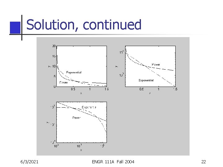
Solution, continued 6/3/2021 ENGR 111 A Fall 2004 22

5. 4 The Plot Editor (p. 292) n n Sometimes it may be easier to work on plots using the plot function, etc. The Plot Editor is a good way to move text around, alter plot scales, add tick marks, etc. Rotating plots is VERY tricky. Read through pages 292 -298 and practice the various features. 6/3/2021 ENGR 111 A Fall 2004 23

5. 4 The Plot Editor (contd. ) n n Practice copying a figure (use one that you have just created) and paste it in a Word file. Use the Copy Figure option in the Edit menu on the figure window. 6/3/2021 ENGR 111 A Fall 2004 24

5. 8 3 -D Plots (p. 334) n n 3 -D plots are a lot like 2 -D plots; just add the z-axis parameters. There are three kinds of 3 -D plots: n n Three Dimensional Line Plots (p. 334). Surface Mesh Plots (p. 335). Contour Plots (p. 337). 3 -D plot functions are in Table 5. 8 -1 (p. 338). 6/3/2021 ENGR 111 A Fall 2004 25

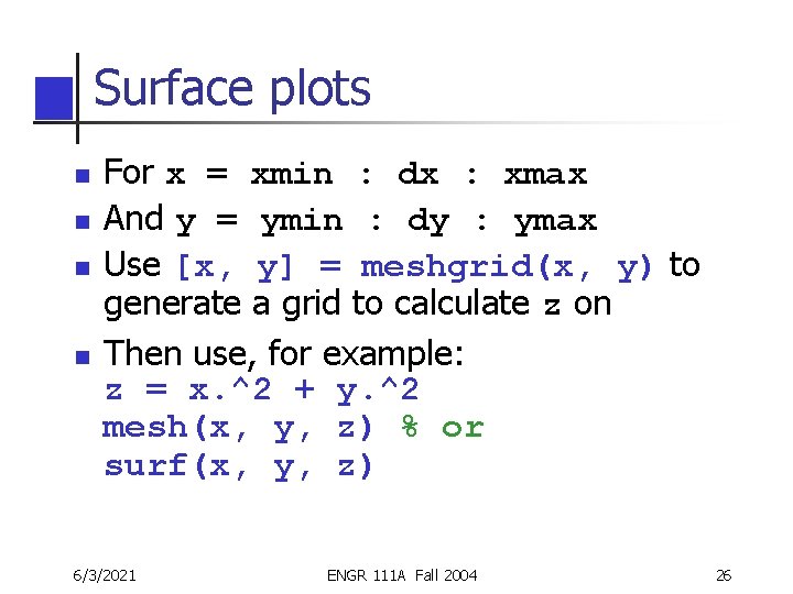
Surface plots n n For x = xmin : dx : xmax And y = ymin : dy : ymax Use [x, y] = meshgrid(x, y) to generate a grid to calculate z on Then use, for example: z = x. ^2 + y. ^2 mesh(x, y, z) % or surf(x, y, z) 6/3/2021 ENGR 111 A Fall 2004 26

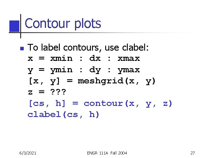
Contour plots n To label contours, use clabel: x = xmin : dx : xmax y = ymin : dy : ymax [x, y] = meshgrid(x, y) z = ? ? ? [cs, h] = contour(x, y, z) clabel(cs, h) 6/3/2021 ENGR 111 A Fall 2004 27

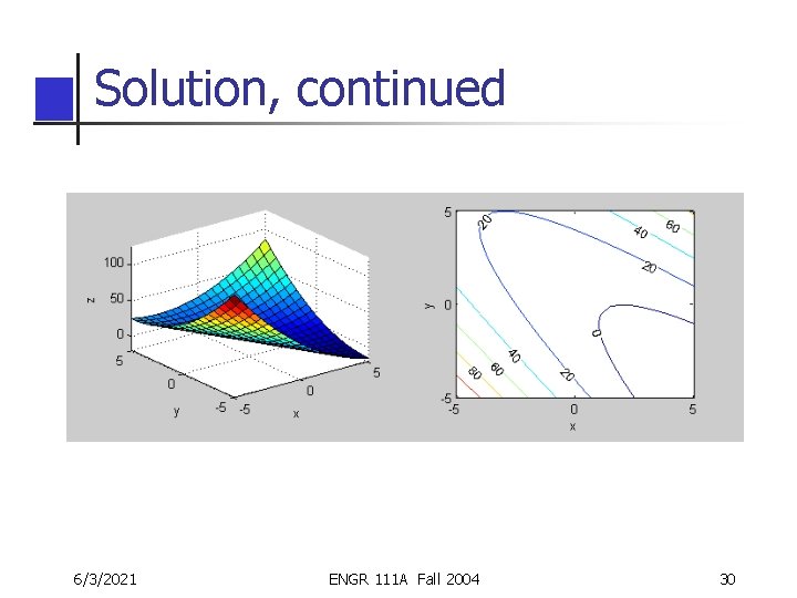
In-Class Exercise 13. 1 -4 (10 -min) n Finally, work T 5. 8 -1 on p. 339. Plot the data for x & y values from -5 to 5 in 0. 5 increments and the z values from -20 to 125. Be sure to label the contours on the contour plot. 6/3/2021 ENGR 111 A Fall 2004 28

Solution [x, y] = meshgrid(-5: 0. 5: 5) z = (x-2). ^2 + 2*x. *y + y. ^2; subplot(2, 2, 1) surf(x, y, z) xlabel('x') ylabel('y') zlabel('z') axis([-5 5 -20 125]) subplot(2, 2, 2) [cs, h] = contour(x, y, z) xlabel('x') ylabel('y') clabel(cs, h) 6/3/2021 ENGR 111 A Fall 2004 29

Solution, continued 6/3/2021 ENGR 111 A Fall 2004 30

Assignment 13. 1 Individual assignment. n Palm Mat. Lab – Chapter 5 (starting on p. 344): # 19, 25, 50. n Due: In one week. n Reading Assignment – Sections 5. 5 to 5. 7. n 6/3/2021 ENGR 111 A Fall 2004 31