Markowitz efficient frontier Econophysics Economics Haichen 4302015 Assumptions

Markowitz efficient frontier Econophysics Economics Haichen 4/30/2015

Assumptions of Markowitz Portfolio Theory 1. Investors consider each investment alternative as being presented by a probability distribution of expected returns over some holding period. 2. Investors minimize one-period expected utility, and their utility curves demonstrate diminishing marginal utility of wealth. 3. Investors estimate the risk of the portfolio on the basis of the variability of expected returns.

Assumptions of Markowitz Portfolio Theory 4. Investors base decisions solely on expected return and risk, so their utility curves are a function of expected return and the expected variance (or standard deviation) of returns only. 5. For a given risk level, investors prefer higher returns to lower returns. Similarly, for a given level of expected returns, investors prefer less risk to more risk.

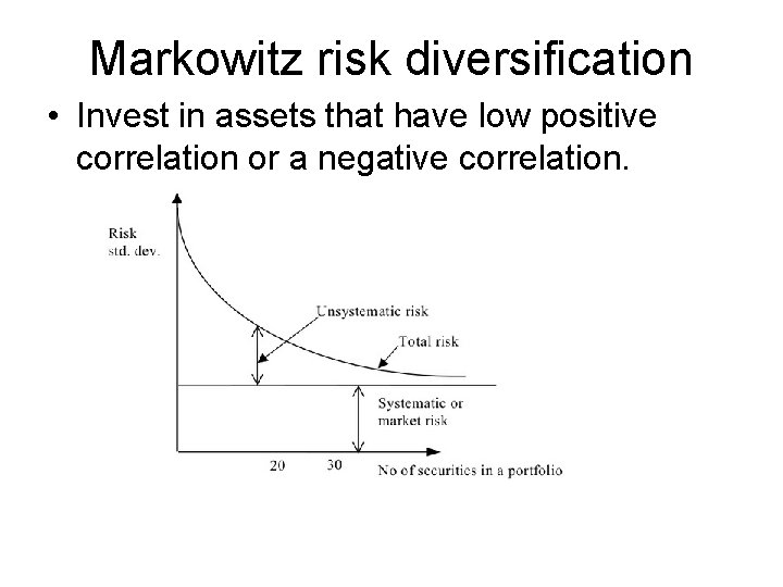
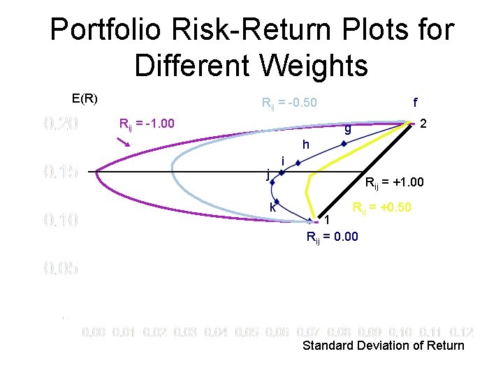
Markowitz risk diversification • Invest in assets that have low positive correlation or a negative correlation.

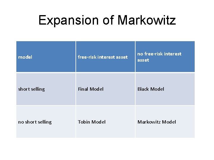
Expansion of Markowitz model free-risk interest asset no free-risk interest asset short selling Final Model Black Model no short selling Tobin Model Markowitz Model

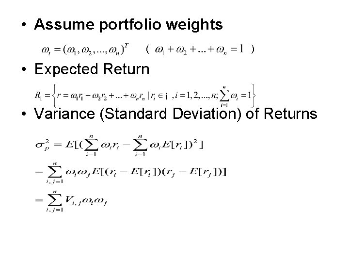
• Assume portfolio weights ( ) • Expected Return • Variance (Standard Deviation) of Returns

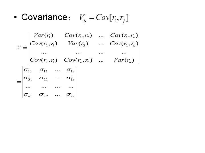
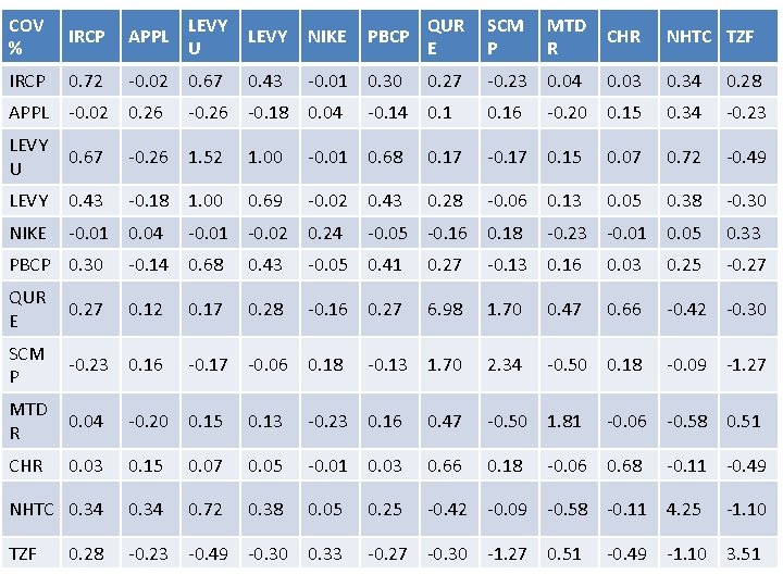
• Covariance：

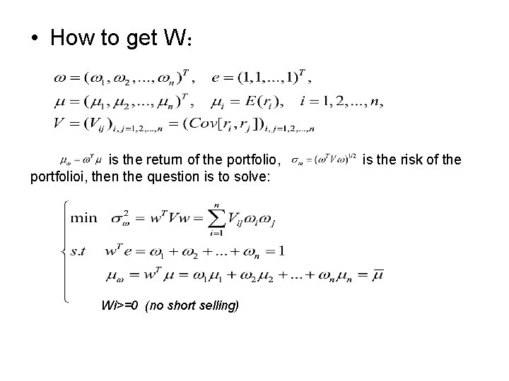
• How to get W： is the return of the portfolio, portfolioi, then the question is to solve: Wi>=0 (no short selling) is the risk of the

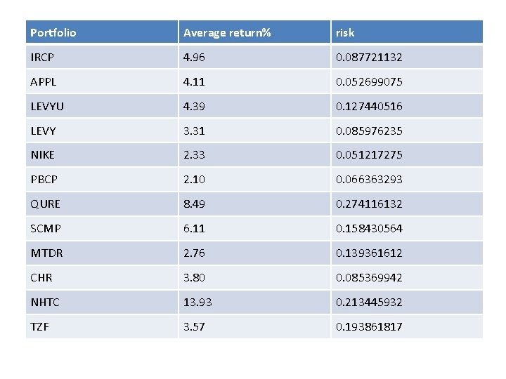
Portfolio Average return% risk IRCP 4. 96 0. 087721132 APPL 4. 11 0. 052699075 LEVYU 4. 39 0. 127440516 LEVY 3. 31 0. 085976235 NIKE 2. 33 0. 051217275 PBCP 2. 10 0. 066363293 QURE 8. 49 0. 274116132 SCMP 6. 11 0. 158430564 MTDR 2. 76 0. 139361612 CHR 3. 80 0. 085369942 NHTC 13. 93 0. 213445932 TZF 3. 57 0. 193861817

COV % IRCP APPL LEVY U LEVY NIKE IRCP 0. 72 -0. 02 0. 67 0. 43 -0. 01 0. 30 APPL -0. 02 0. 26 LEVY U 0. 67 -0. 26 1. 52 1. 00 -0. 01 0. 68 0. 17 -0. 17 0. 15 LEVY 0. 43 -0. 18 1. 00 0. 69 -0. 02 0. 43 0. 28 -0. 06 0. 13 NIKE -0. 01 0. 04 -0. 26 -0. 18 0. 04 -0. 01 -0. 02 0. 24 PBCP QUR E SCM P MTD R CHR NHTC TZF 0. 27 -0. 23 0. 04 0. 03 0. 34 0. 28 -0. 20 0. 15 0. 34 -0. 23 0. 07 0. 72 -0. 49 0. 05 0. 38 -0. 30 -0. 14 0. 16 -0. 05 -0. 16 0. 18 -0. 23 -0. 01 0. 05 0. 33 PBCP 0. 30 -0. 14 0. 68 0. 43 -0. 05 0. 41 0. 27 -0. 13 0. 16 0. 03 0. 25 QUR E 0. 27 0. 12 0. 28 -0. 16 0. 27 6. 98 1. 70 0. 47 0. 66 -0. 42 -0. 30 SCM P -0. 23 0. 16 -0. 13 1. 70 2. 34 -0. 50 0. 18 -0. 09 -1. 27 MTD R 0. 04 -0. 20 0. 15 0. 13 -0. 23 0. 16 0. 47 -0. 50 1. 81 CHR 0. 03 0. 15 0. 07 0. 05 -0. 01 0. 03 0. 66 0. 18 NHTC 0. 34 0. 72 0. 38 0. 05 -0. 42 -0. 09 -0. 58 -0. 11 4. 25 TZF -0. 23 -0. 49 -0. 30 0. 33 0. 28 0. 17 -0. 06 0. 18 0. 25 -0. 06 -0. 58 0. 51 -0. 06 0. 68 -0. 27 -0. 30 -1. 27 0. 51 -0. 27 -0. 11 -0. 49 -1. 10 3. 51

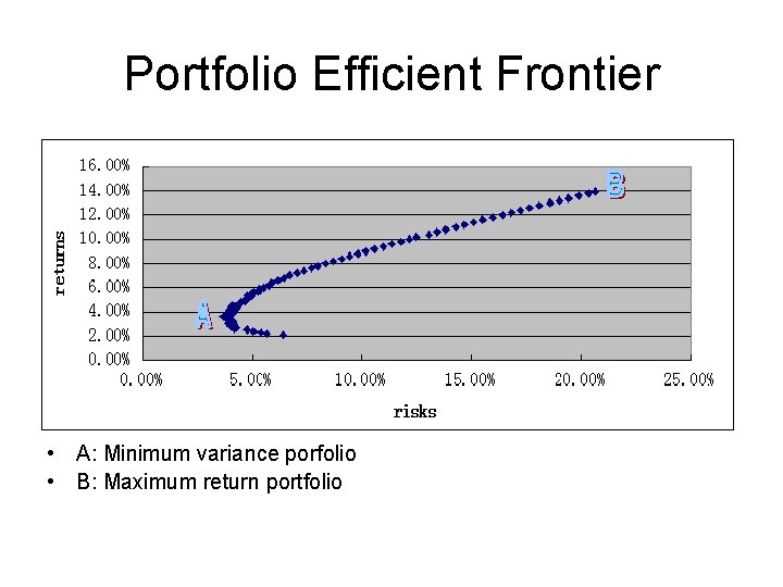
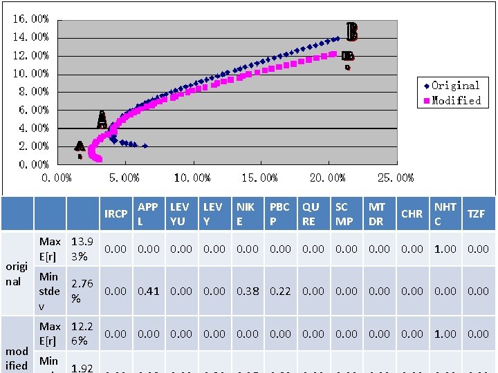
Portfolio Efficient Frontier • A: Minimum variance porfolio • B: Maximum return portfolio

Portfolio Risk-Return Plots for Different Weights E(R) Rij = -0. 50 Rij = -1. 00 f 2 g h j k i Rij = +1. 00 Rij = +0. 50 1 Rij = 0. 00 Standard Deviation of Return

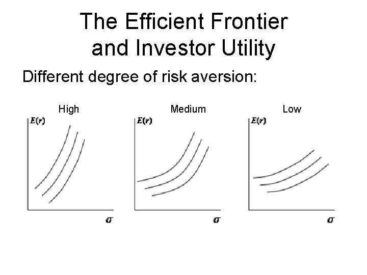
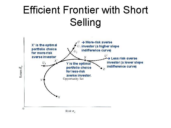
The Efficient Frontier and Investor Utility Different degree of risk aversion: High Medium Low

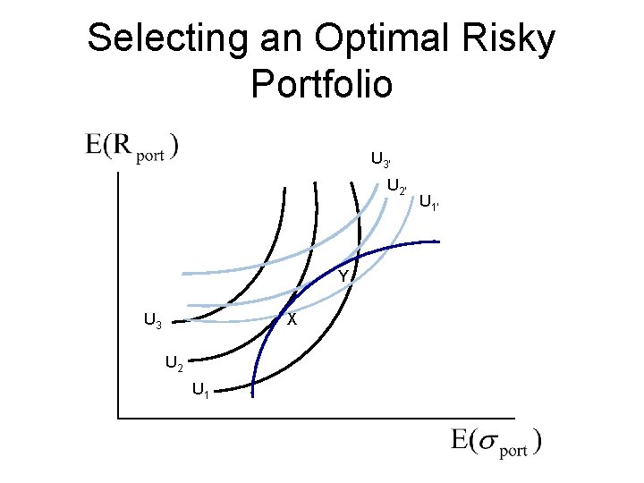
Selecting an Optimal Risky Portfolio U 3’ U 2’ Y U 3 X U 2 U 1’

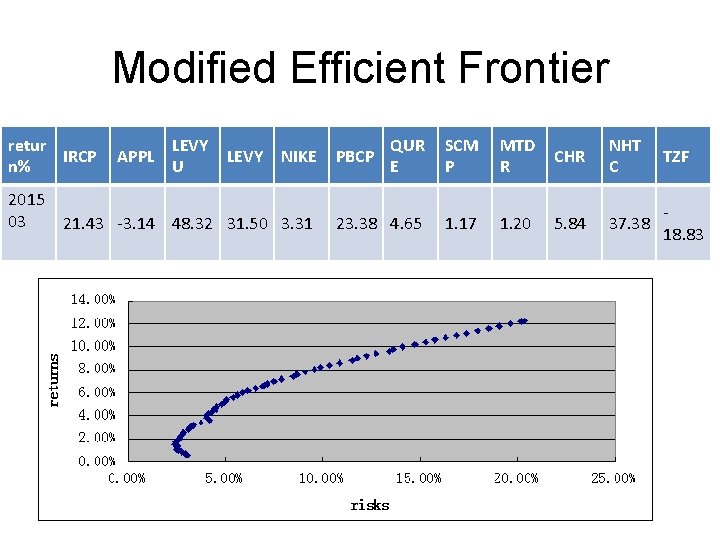
Modified Efficient Frontier retur IRCP n% 2015 03 APPL LEVY U LEVY NIKE 21. 43 -3. 14 48. 32 31. 50 3. 31 QUR E SCM P MTD R CHR NHT C TZF 23. 38 4. 65 1. 17 1. 20 5. 84 37. 38 18. 83 PBCP

IRCP APP LEV L YU LEV Y NIK E PBC P QU RE SC MP MT DR CHR NHT TZF C Max 13. 9 0. 00 0. 00 1. 00 0. 00 E[r] 3% origi nal Min 2. 76 stde 0. 00 0. 41 0. 00 0. 38 0. 22 0. 00 % v Max 12. 2 0. 00 0. 00 1. 00 0. 00 E[r] 6% mod ified Min 1. 92

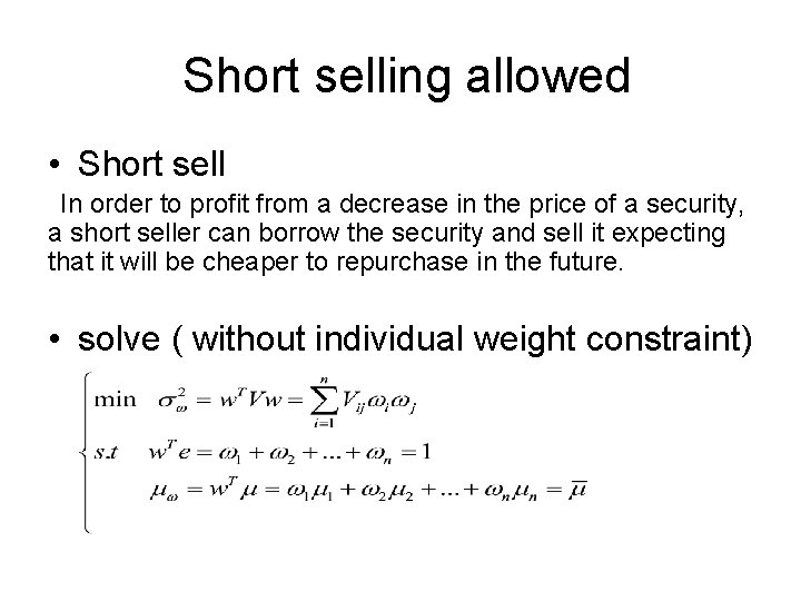
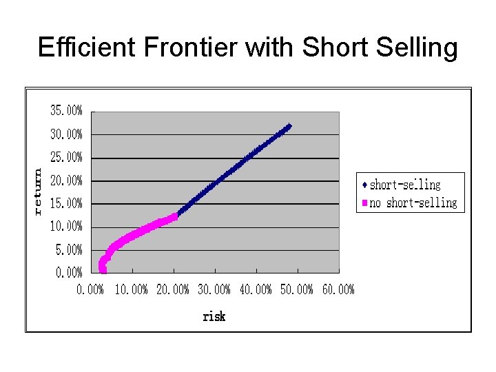
Short selling allowed • Short sell In order to profit from a decrease in the price of a security, a short seller can borrow the security and sell it expecting that it will be cheaper to repurchase in the future. • solve ( without individual weight constraint)

Efficient Frontier with Short Selling

Efficient Frontier with Short Selling X’ is the optimal portfolio choice for more-risk averse investor More-risk averse investor (a higher slope indifference curve) Y is the optimal portfolio choice for less-risk averse investor. Less risk-averse investor (a lower slope indifference curve)

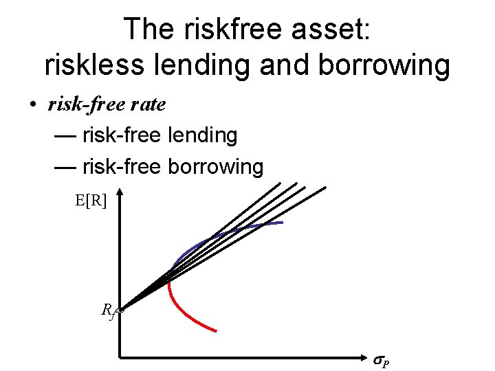
The riskfree asset: riskless lending and borrowing • risk-free rate — risk-free lending — risk-free borrowing E[R] Rf P

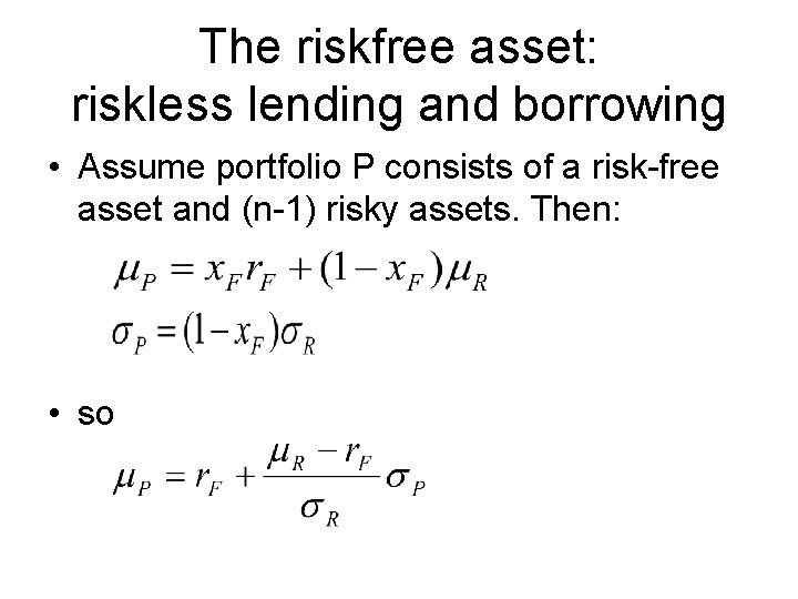
The riskfree asset: riskless lending and borrowing • Assume portfolio P consists of a risk-free asset and (n-1) risky assets. Then: • so

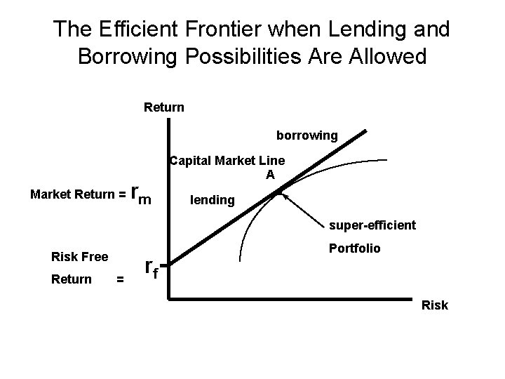
The Efficient Frontier when Lending and Borrowing Possibilities Are Allowed Return borrowing Capital Market Line A r Market Return = m lending . super-efficient Risk Free Return = rf Portfolio Risk

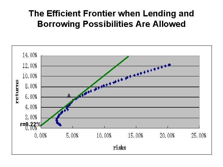
The Efficient Frontier when Lending and Borrowing Possibilities Are Allowed A r=0. 22%

Thank you • Thanks for Chester and Antonio's help.