Markov Models 1 Review Markov Process Bayes formula

Markov Models 1
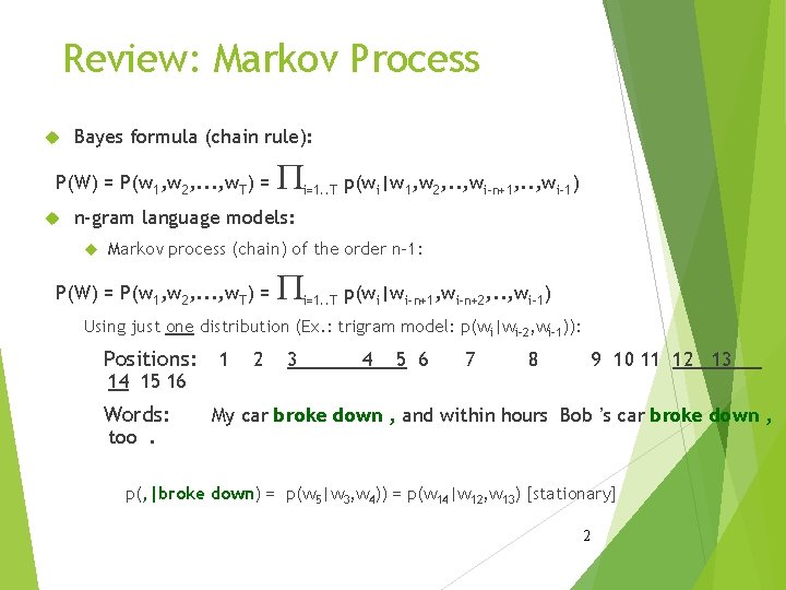
Review: Markov Process Bayes formula (chain rule): P(W) = P(w 1, w 2, . . . , w. T) = P i=1. . T p(wi|w 1, w 2, . . , wi-n+1, . . , wi-1) n-gram language models: Markov process (chain) of the order n-1: P(W) = P(w 1, w 2, . . . , w. T) = P i=1. . T p(wi|wi-n+1, wi-n+2, . . , wi-1) Using just one distribution (Ex. : trigram model: p(wi|wi-2, wi-1)): Positions: 1 14 15 16 Words: too. 2 3 4 5 6 7 8 9 10 11 12 13 My car broke down , and within hours Bob ’s car broke down , p(, |broke down) = p(w 5|w 3, w 4)) = p(w 14|w 12, w 13) [stationary] 2
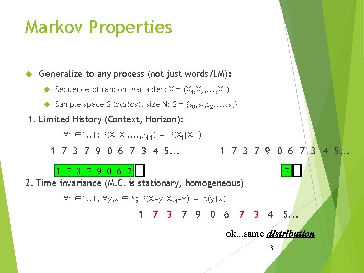
Markov Properties Generalize to any process (not just words/LM): Sequence of random variables: X = (X 1, X 2, . . . , XT) Sample space S (states), size N: S = {s 0, s 1, s 2, . . . , s. N} 1. Limited History (Context, Horizon): "i ∈1. . T; P(Xi|X 1, . . . , Xi-1) = P(Xi|Xi-1) 1 7 3 7 9 0 6 7 3 4 5. . . 7 1 7 3 7 9 0 6 7 2. Time invariance (M. C. is stationary, homogeneous) "i ∈1. . T, "y, x ∈ S; P(Xi=y|Xi-1=x) = p(y|x) 1 7 3 7 9 0 6 7 3 4 5. . . ok. . . same distribution 3
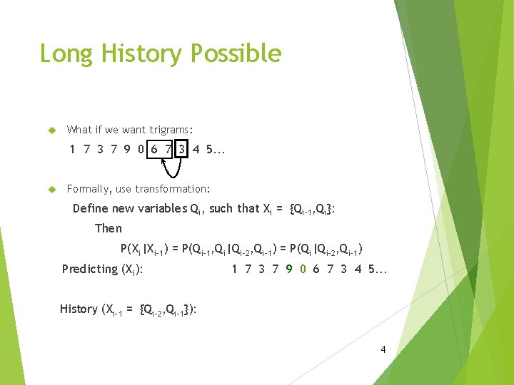
Long History Possible What if we want trigrams: 1 7 3 7 9 0 6 7 3 4 5. . . Formally, use transformation: Define new variables Qi, such that Xi = {Qi-1, Qi}: Then P(Xi|Xi-1) = P(Qi-1, Qi|Qi-2, Qi-1) = P(Qi|Qi-2, Qi-1) Predicting (Xi): 1 7 3 7 9 0 6 7 3 4 5. . . History (Xi-1 = {Qi-2, Qi-1}): 4
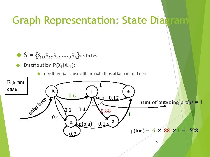
Graph Representation: State Diagram S = {s 0, s 1, s 2, . . . , s. N}: states Distribution P(Xi|Xi-1): transitions (as arcs) with probabilities attached to them: Bigram case: ⅹ e er te n e rh 1 0. 3 0. 4 t 0. 6 a 0. 2 0. 4 e 0. 12 0. 88 sum of outgoing probs = 1 1 p(o|a) = 0. 1 o p(toe) =. 6 ⅹ. 88 ⅹ 1 =. 528 5
![Finite State Automaton States ~ symbols of the [input/output] alphabet Arcs ~ transitions (sequence Finite State Automaton States ~ symbols of the [input/output] alphabet Arcs ~ transitions (sequence](http://slidetodoc.com/presentation_image_h2/f7d7b5d045a6f6f425a2fc1144e353cd/image-6.jpg)
Finite State Automaton States ~ symbols of the [input/output] alphabet Arcs ~ transitions (sequence of states) [Classical FSA: alphabet symbols on arcs: transformation: arcs ↔ nodes] So far: Visible Markov Models (VMM) 6
![Hidden Markov Models The simplest HMM: states generate [observable] output (using the “data” alphabet) Hidden Markov Models The simplest HMM: states generate [observable] output (using the “data” alphabet)](http://slidetodoc.com/presentation_image_h2/f7d7b5d045a6f6f425a2fc1144e353cd/image-7.jpg)
Hidden Markov Models The simplest HMM: states generate [observable] output (using the “data” alphabet) but remain “invisible”: t e Reverse arrow! x er t en e er h 1 0. 3 0. 4 a 1 0. 6 3 0. 2 0. 4 2 0. 12 0. 88 1 p(4|3) = 0. 1 4 p(toe) =. 6 x. 88 x 1 =. 528 o 7
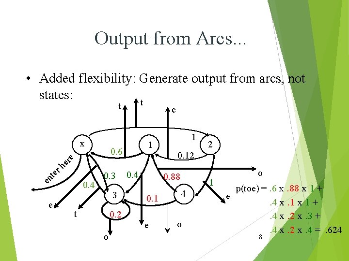
Output from Arcs. . . • Added flexibility: Generate output from arcs, not states: t t x te n e e 0. 4 1 0. 6 re e h r e 0. 3 3 t 0. 4 0. 1 e 2 0. 12 0. 88 0. 2 o 1 1 4 o o p(toe) =. 6 x. 88 x 1 + e. 4 x. 1 x 1 +. 4 x. 2 x. 3 +. 4 x. 2 x. 4 =. 624 8
![. . . and Finally, Add Output Probabilities • Maximum flexibility: [Unigram] distribution (sample . . . and Finally, Add Output Probabilities • Maximum flexibility: [Unigram] distribution (sample](http://slidetodoc.com/presentation_image_h2/f7d7b5d045a6f6f425a2fc1144e353cd/image-9.jpg)
. . . and Finally, Add Output Probabilities • Maximum flexibility: [Unigram] distribution (sample space: output alphabet) at each output arc: p(t)=0 p(o)=0 p(e)=1 p(t)=. 8 p(o)=. 1 p(e)=. 1 x re te n e e h r 1 0. 6 1 0. 4 3 p(t)=. 5 p(o)=. 2 p(e)=. 3 0. 88 p(t)=0 p(o)=1 p(e)=0 2 0. 12 4 1 p(t)=. 1 p(o)=. 7 p(e)=. 2 p(toe) =. 6 x. 88 x. 7 x 1 x. 6 +. 4 x. 5 x 1 x 1 x. 88 x. 2 + p(t)=0. 4 x. 5 x 1 x 1 x. 12 x 1 p(o)=. 4 @. 237 p(e)=. 6 9
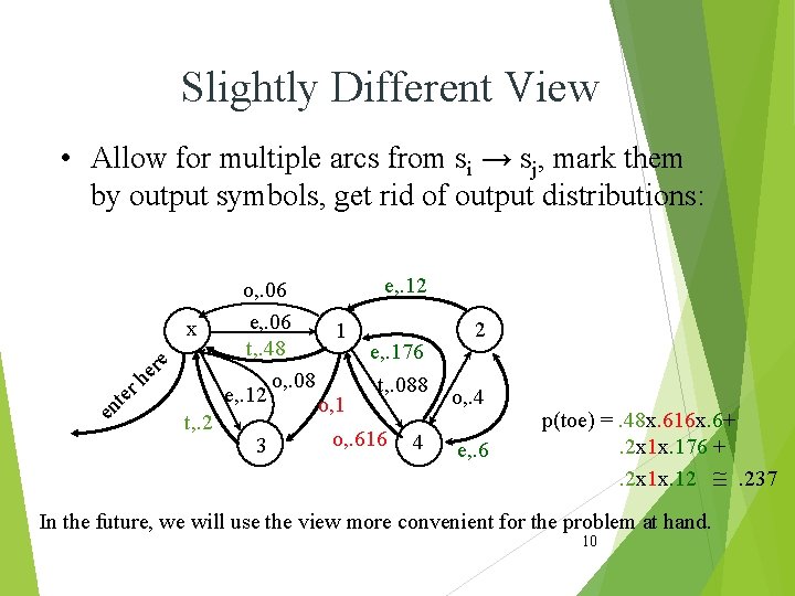
Slightly Different View • Allow for multiple arcs from si → sj, mark them by output symbols, get rid of output distributions: x e er h r e t en t, . 2 o, . 06 e, . 06 1 t, . 48 o, . 08 e, . 12 o, 1 3 e, . 12 e, . 176 t, . 088 o, . 616 4 2 o, . 4 e, . 6 p(toe) =. 48 x. 616 x. 6+. 2 x 1 x. 176 +. 2 x 1 x. 12 @. 237 In the future, we will use the view more convenient for the problem at hand. 10
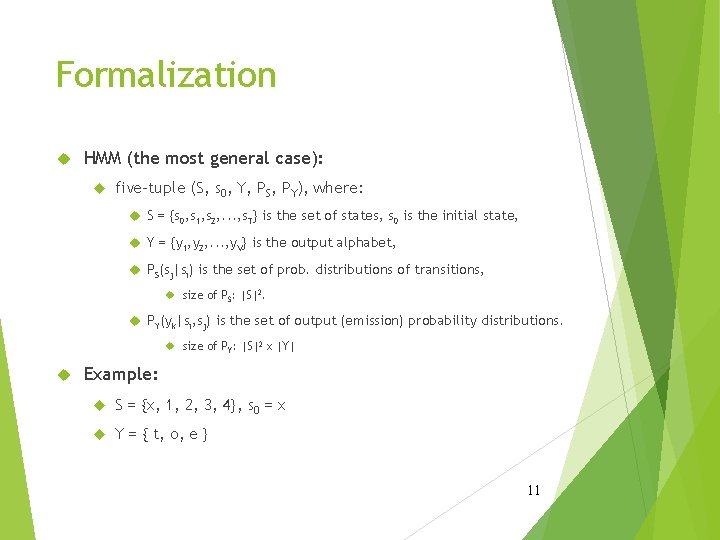
Formalization HMM (the most general case): five-tuple (S, s 0, Y, PS, PY), where: S = {s 0, s 1, s 2, . . . , s. T} is the set of states, s 0 is the initial state, Y = {y 1, y 2, . . . , y. V} is the output alphabet, PS(sj|si) is the set of prob. distributions of transitions, size of PS: |S|2. PY(yk|si, sj) is the set of output (emission) probability distributions. size of PY: |S|2 x |Y| Example: S = {x, 1, 2, 3, 4}, s 0 = x Y = { t, o, e } 11
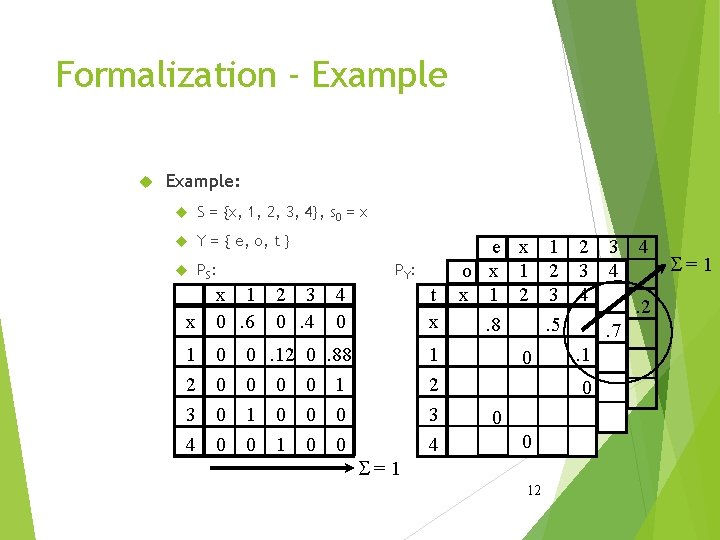
Formalization - Example: S = {x, 1, 2, 3, 4}, s 0 = x Y = { e, o, t } PS : PY: x x 1 0. 6 1 2 3 4 0 0 2 3 0. 4 4 0 0. 12 0. 88 0 0 0 1 1 0 0 t x S=1 1 2 3 4 o x 1 2 3 4 e x 1 2 3 4 S=1 x 1 2 3 4 1. 2. 8. 5. 7 2. 1 3 0 0 4 0 0 12
Using the HMM The generation algorithm (of limited value : -)): 1. Start in s = s 0. 2. Move from s to s’ with probability PS(s’|s). 3. Output (emit) symbol yk with probability PS(yk|s, s’). 4. Repeat from step 2 (until somebody says enough). More interesting usage: Given an output sequence Y = {y 1, y 2, . . . , yk}, compute its probability. Given an output sequence Y = {y 1, y 2, . . . , yk}, compute the most likely sequence of states which has generated it. . plus variations: e. g. , n best state sequences 13
HMM Algorithms: Trellis and Viterbi 14
HMM: The Two Tasks HMM (the general case): five-tuple (S, S 0, Y, PS, PY), where: S = {s 1, s 2, . . . , s. T} is the set of states, S 0 is the initial state, Y = {y 1, y 2, . . . , y. V} is the output alphabet, PS(sj|si) is the set of prob. distributions of transitions, PY(yk|si, sj) is the set of output (emission) probability distributions. Given an HMM & an output sequence Y = {y 1, y 2, . . . , yk}: (Task 1) compute the probability of Y; (Task 2) compute the most likely sequence of states which has generated Y. 15
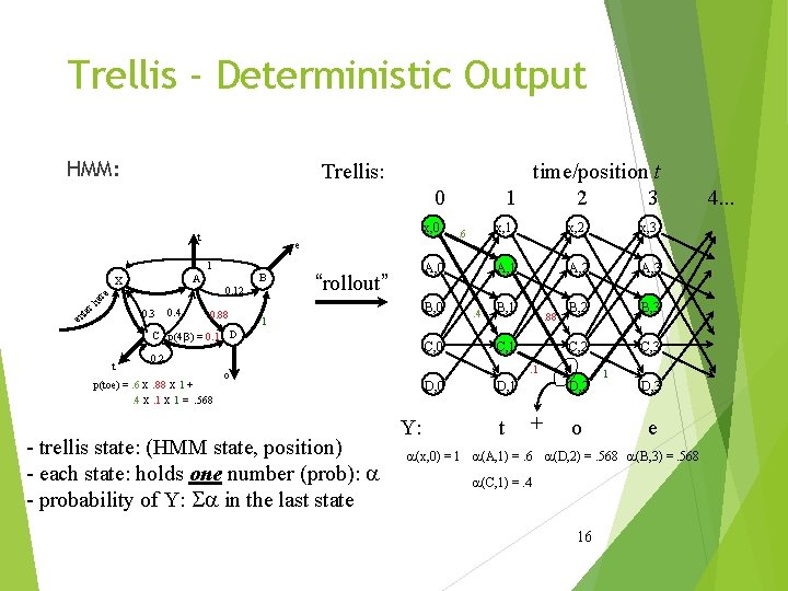
Trellis - Deterministic Output HMM: Trellis: time/position t 1 2 3 0 x, 0 t e er rh 1 x e t en e B A 0. 3 0. 4 0. 12 0. 88 A, 0 “rollout” B, 0 1 C p(4|3) = 0. 1 D t C, 0 0. 2 p(toe) =. 6 x. 88 x 1 +. 4 x. 1 x 1 =. 568 . 4 x, 1 x, 2 x, 3 A, 1 A, 2 A, 3 B, 2 B, 3 C, 2 C, 3 B, 1 . 88 C, 1. 1 o - trellis state: (HMM state, position) - each state: holds one number (prob): a - probability of Y: Sa in the last state . 6 D, 0 Y: D, 1 t D, 2 + o 1 D, 3 e a(x, 0) = 1 a(A, 1) =. 6 a(D, 2) =. 568 a(B, 3) =. 568 a(C, 1) =. 4 16 4. . .
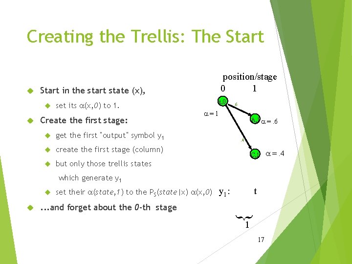
Creating the Trellis: The Start in the start state (x), position/stage 0 1 set its a(x, 0) to 1. Create the first stage: get the first “output” symbol y 1 create the first stage (column) but only those trellis states x, 0 . 6 a=1 A, 1 a =. 6. 4 C, 1 which generate y 1 set their a(state, 1) to the PS(state|x) a(x, 0) y 1: t . . . and forget about the 0 -th stage } 1 17 a =. 4
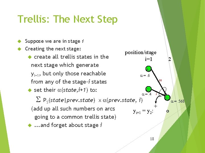
Trellis: The Next Step Suppose we are in stage i Creating the next stage: create all trellis states in the next stage which generate yi+1, but only those reachable from any of the stage-i states set their a(state, i+1) to: S position/stage i=1 A, 1 a =. 6. 88 C, 1 a =. 4 . 1 D, 2 PS(state|prev. state) ⅹa(prev. state, i) (add up all such numbers on arcs going to a common trellis state) . . . and forget about stage i 2 yi+1 = y 2: 18 + o a =. 568
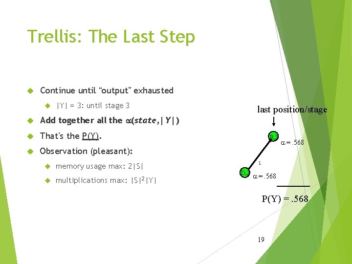
Trellis: The Last Step Continue until “output” exhausted |Y| = 3: until stage 3 Add together all the a(state, |Y|) That’s the P(Y). Observation (pleasant): B, 3 memory usage max: 2|S| multiplications max: last position/stage |S|2|Y| a =. 568 1 D, 2 a =. 568 P(Y) =. 568 19
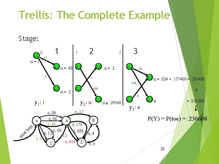
Trellis: The Complete Example Stage: x, 0 1 0 a=1 2 1 3 2 . 48 A, 2 a =. 2 A, 1 a =. 48 A, 1. 2 A, 2 . 12 B, 3 a =. 024 +. 177408 =. 201408 1. 176 C, 1 a =. 2 + . 616 C, 1 . 6 y 1: t x en te e er h r t, . 2 D, 2 y 2: o e, . 12 o, . 06 e, . 06 A t, . 48 e, . 176 o, . 08 t, . 088 e, . 12 o, 1 C o, . 616 D B a @. 29568 D, 2 D, 3 a =. 035200 y 3: e P(Y) = P(toe) =. 236608 o, . 4 e, . 6 20
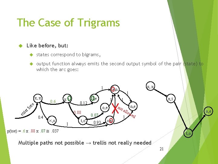
The Case of Trigrams Like before, but: states correspond to bigrams, output function always emits the second output symbol of the pair (state) to which the arc goes: 1 x, x e er h r 0. 6 xt te en 0. 12 0. 88 0. 4 ´, o 1 t, o t, e 1 1 o, e 0. 07 0. 93 x, x e, n o, n x, t 1 no n, e t al 1 o, e low ed p(toe) =. 6 x. 88 x. 07 @. 037 t, o Multiple paths not possible → trellis not really needed 21
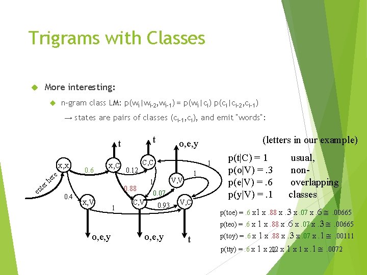
Trigrams with Classes More interesting: n-gram class LM: p(wi|wi-2, wi-1) = p(wi|ci) p(ci|ci-2, ci-1) → states are pairs of classes (ci-1, ci), and emit “words”: t t x, x e er nt re he 0. 6 x, C C, C 0. 4 x, V o, e, y 1 1 0. 12 1 V, V 1 0. 88 0. 07 C, V (letters in our example) o, e, y 0. 93 o, e, y V, C p(t|C) = 1 p(o|V) =. 3 p(e|V) =. 6 p(y|V) =. 1 usual, nonoverlapping classes p(toe) =. 6 x 1 x. 88 x t . 3 x. 07 x. 6 @. 00665 p(teo) =. 6 x 1 x. 88 x. 6 x. 07 x. 3 @. 00665 p(toy) =. 6 x 1 x. 88 x. 3 x. 07 x. 1 @. 00111 p(tty) =. 6 x 1 x 22. 12 x 1 x. 1 @. 0072
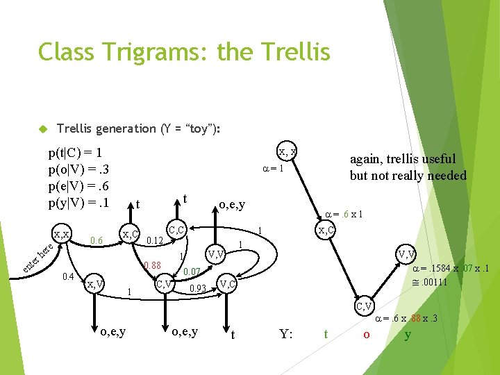
Class Trigrams: the Trellis generation (Y = “toy”): x, x p(t|C) = 1 p(o|V) =. 3 p(e|V) =. 6 p(y|V) =. 1 x, x e er h r 0. 6 t t x, C te en x, V 1 o, e, y C, C a =. 6 x 1 x, C 1 0. 12 1 V, V 1 0. 88 0. 4 again, trellis useful but not really needed a=1 V, V a =. 1584 x. 07 x. 1 @. 00111 0. 07 C, V 0. 93 V, C C, V o, e, y t Y: t o a =. 6 x. 88 x. 3 y
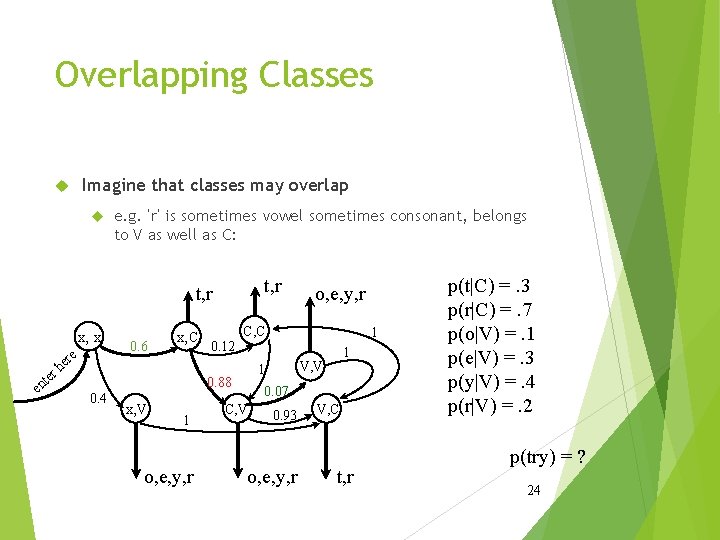
Overlapping Classes Imagine that classes may overlap e. g. ‘r’ is sometimes vowel sometimes consonant, belongs to V as well as C: t, r x, x te en e er h r 0. 6 x, C C, C x, V 1 o, e, y, r 1 0. 12 1 V, V 1 0. 88 0. 4 o, e, y, r 0. 07 C, V 0. 93 o, e, y, r V, C t, r p(t|C) =. 3 p(r|C) =. 7 p(o|V) =. 1 p(e|V) =. 3 p(y|V) =. 4 p(r|V) =. 2 p(try) = ? 24
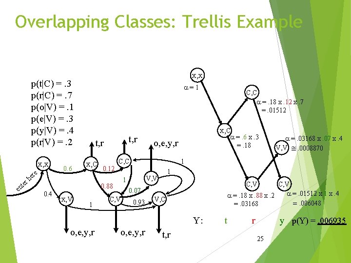
Overlapping Classes: Trellis Example x, x p(t|C) =. 3 p(r|C) =. 7 p(o|V) =. 1 p(e|V) =. 3 p(y|V) =. 4 p(r|V) =. 2 x, x r te en re he 0. 6 a=1 t, r x, C 0. 4 x, V 1 x, C a =. 6 x. 3 =. 18 o, e, y, r 0. 12 1 V, V 1 C, V a =. 01512 x 1 x. 4 a =. 18 x. 88 x. 2 =. 006048 =. 03168 0. 07 C, V 0. 93 V, C Y: o, e, y, r a =. 03168 x. 07 x. 4 V, V @. 0008870 1 C, C 0. 88 C, C a =. 18 x. 12 x. 7 =. 01512 o, e, y, r t r y p(Y) =. 006935 25
Trellis: Remarks So far, we went left to right (computing a) Same result: going right to left (computing b) supposed we know where to start (finite data) In fact, we might start in the middle going left and right Important for parameter estimation (Forward-Backward Algortihm alias Baum-Welch) Implementation issues: scaling/normalizing probabilities, to avoid too small numbers & addition problems with many transitions 26
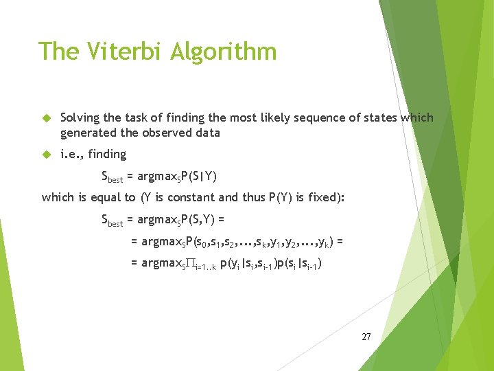
The Viterbi Algorithm Solving the task of finding the most likely sequence of states which generated the observed data i. e. , finding Sbest = argmax. SP(S|Y) which is equal to (Y is constant and thus P(Y) is fixed): Sbest = argmax. SP(S, Y) = = argmax. SP(s 0, s 1, s 2, . . . , sk, y 1, y 2, . . . , yk) = = argmax. SPi=1. . k p(yi|si, si-1)p(si|si-1) 27
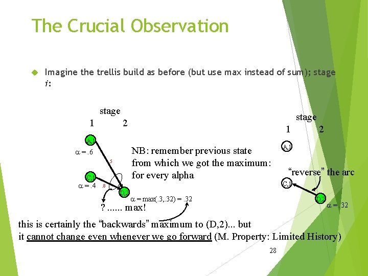
The Crucial Observation Imagine the trellis build as before (but use max instead of sum); stage i: stage 1 stage 2 1 A, 1 NB: remember previous state from which we got the maximum: for every alpha a =. 6. 5 C, 1 a =. 4 . 8 D, 2 a = max(. 3, . 32) =. 32 2 A, 1 “reverse” the arc C, 1 D, 2 ? . . . max! a =. 32 this is certainly the “backwards” maximum to (D, 2). . . but it cannot change even whenever we go forward (M. Property: Limited History) 28
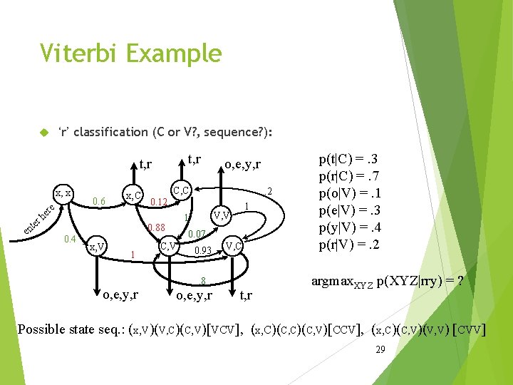
Viterbi Example ‘r’ classification (C or V? , sequence? ): t, r x, x e r te n e r he 0. 6 x, C C, C x, V 1 o, e, y, r . 2 0. 12 1 V, V 1 0. 88 0. 4 o, e, y, r 0. 07 C, V 0. 93 V, C . 8 o, e, y, r t, r p(t|C) =. 3 p(r|C) =. 7 p(o|V) =. 1 p(e|V) =. 3 p(y|V) =. 4 p(r|V) =. 2 argmax. XYZ p(XYZ|rry) = ? Possible state seq. : (x, V)(V, C)(C, V)[VCV], (x, C)(C, V)[CCV], (x, C)(C, V)(V, V) [CVV] 29
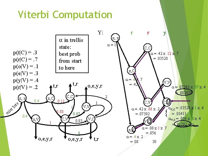
Viterbi Computation Y: p(t|C) =. 3 p(r|C) =. 7 p(o|V) =. 1 p(e|V) =. 3 p(y|V) =. 4 p(r|V) =. 2 x, x r te en re he 0. 6 t, r x, C x, V 1 o, e, y, r a=1 y C, C a =. 42 x. 12 x. 7 =. 03528 a =. 6 x. 7 =. 42 o, e, y, r V, V . 2 0. 12 1 V, V 1 0. 07 C, V r x, C C, C 0. 88 0. 4 x, x a in trellis state: best prob from start to here r 0. 93 V, C . 8 o, e, y, r t, r C, V a =. 07392 x. 07 x. 4 =. 002070 C, V a. C, C =. 03528 x 1 x. 4 a =. 42 x. 88 x. 2 =. 01411 =. 07392 a. V, C =. 056 x. 8 x. 4 V, C =. 01792 = amax a =. 08 x 1 x. 7 x, V =. 056 a =. 4 x. 2 =. 08 30 {
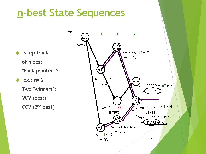
n-best State Sequences Y: x, x r a=1 r C, C Keep track a =. 42 x. 12 x. 7 =. 03528 of n best “back pointers”: Ex. : n= 2: x, C a =. 6 x. 7 =. 42 V, V a =. 07392 x. 07 x. 4 =. 002070 Two “winners”: VCV (best) CCV (2 nd best) y C, V a. C, C =. 03528 x 1 x. 4 a =. 42 x. 88 x. 2 =. 07392 ? =. 01411 a. V, C =. 056 x. 8 x. 4 V, C =. 01792 = amax a =. 08 x 1 x. 7 x, V =. 056 a =. 4 x. 2 =. 08 31 {
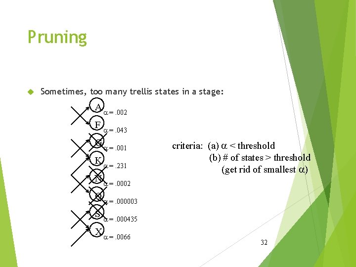
Pruning Sometimes, too many trellis states in a stage: A a =. 002 F a =. 043 G a =. 001 K a =. 231 N a =. 0002 criteria: (a) a < threshold (b) # of states > threshold (get rid of smallest a) Q a =. 000003 S a =. 000435 X a =. 0066 32
HMM Parameter Estimation: the Baum-Welch Algorithm 33
HMM: The Tasks HMM (the general case): five-tuple (S, S 0, Y, PS, PY), where: S = {s 1, s 2, . . . , s. T} is the set of states, S 0 is the initial state, Y = {y 1, y 2, . . . , y. V} is the output alphabet, PS(sj|si) is the set of prob. distributions of transitions, PY(yk|si, sj) is the set of output (emission) probability distributions. Given an HMM & an output sequence Y = {y 1, y 2, . . . , yk}: ü (Task 1) compute the probability of Y; ü (Task 2) compute the most likely sequence of states which has generated Y. (Task 3) Estimating the parameters (transition/output distributions) 34
A Variant of EM Idea (~ EM: Expectation-Maximization): Start with (possibly random) estimates of PS and PY. Compute (fractional) “counts” of state transitions/emissions taken, from PS and PY, given data Y. Adjust the estimates of PS and PY from these “counts” (using the MLE, i. e. relative frequency as the estimate). 35
Setting HMM (without PS, PY) (S, S 0, Y), and data T = {yi∈Y}i=1. . |T| will use T ~ |T| HMM structure is given: (S, S 0) PS: Typically, one wants to allow “fully connected” graph (i. e. no transitions forbidden ~ no transitions set to hard 0) why? → we better leave it on the learning phase, based on the data! sometimes possible to remove some transitions ahead of time PY: should be restricted (if not, we will not get anywhere!) restricted ~ hard 0 probabilities of p(y|s, s’) “Dictionary”: states (e. g. POS tag) ↔ words, “m: n” mapping on SⅹY (in general) 36
Initialization For computing the initial expected “counts” Important part EM guaranteed to find a local maximum only (albeit a good one in most cases) PY initialization more important fortunately, often easy to determine together with dictionary ↔ vocabulary mapping, get counts, then MLE PS initialization less important e. g. uniform distribution for each p(. |s) 37
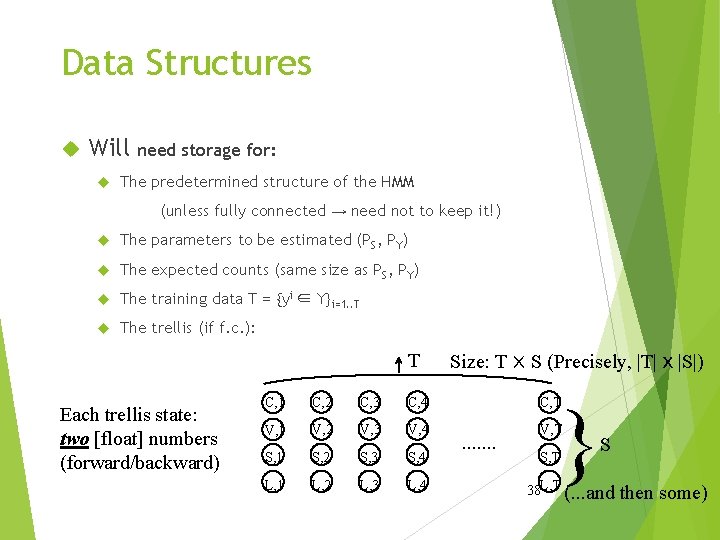
Data Structures Will need storage for: The predetermined structure of the HMM (unless fully connected → need not to keep it!) The parameters to be estimated (PS, PY) The expected counts (same size as PS, PY) The training data T = {yi ∈ Y}i=1. . T The trellis (if f. c. ): T Each trellis state: two [float] numbers (forward/backward) Size: TⅹS (Precisely, |T|ⅹ|S|) } C, 1 C, 2 C, 3 C, 4 C, T V, 1 V, 2 V, 3 V, 4 V, T S, 1 S, 2 S, 3 S, 4 L, 1 L, 2 L, 3 L, 4 . . . . S, T S 38 L, T (. . . and then some)
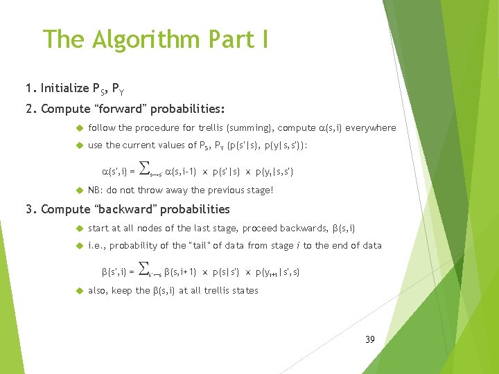
The Algorithm Part I 1. Initialize PS, PY 2. Compute “forward” probabilities: follow the procedure for trellis (summing), compute a(s, i) everywhere use the current values of PS, PY (p(s’|s), p(y|s, s’)): a(s’, i) = S s→s’ a(s, i-1) ⅹ p(s’|s) ⅹ p(yi|s, s’) NB: do not throw away the previous stage! 3. Compute “backward” probabilities start at all nodes of the last stage, proceed backwards, b(s, i) i. e. , probability of the “tail” of data from stage i to the end of data b(s’, i) = S s’←s b(s, i+1) ⅹ p(s|s’) ⅹ p(yi+1|s’, s) also, keep the b(s, i) at all trellis states 39
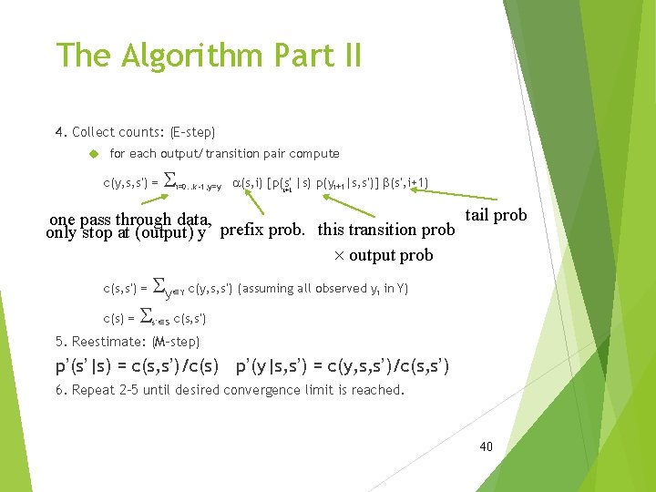
The Algorithm Part II 4. Collect counts: (E-step) for each output/transition pair compute c(y, s, s’) = S i=0. . k-1, y=y a(s, i) [p(s’ |s) p(yi+1|s, s’)] b(s’, i+1) i+1 tail prob one pass through data, only stop at (output) y prefix prob. this transition prob ´ output prob Sy c(y, s, s’) (assuming all observed y in Y) c(s) = S c(s, s’) = ∈Y i s’∈S 5. Reestimate: (M-step) p’(s’|s) = c(s, s’)/c(s) p’(y|s, s’) = c(y, s, s’)/c(s, s’) 6. Repeat 2 -5 until desired convergence limit is reached. 40
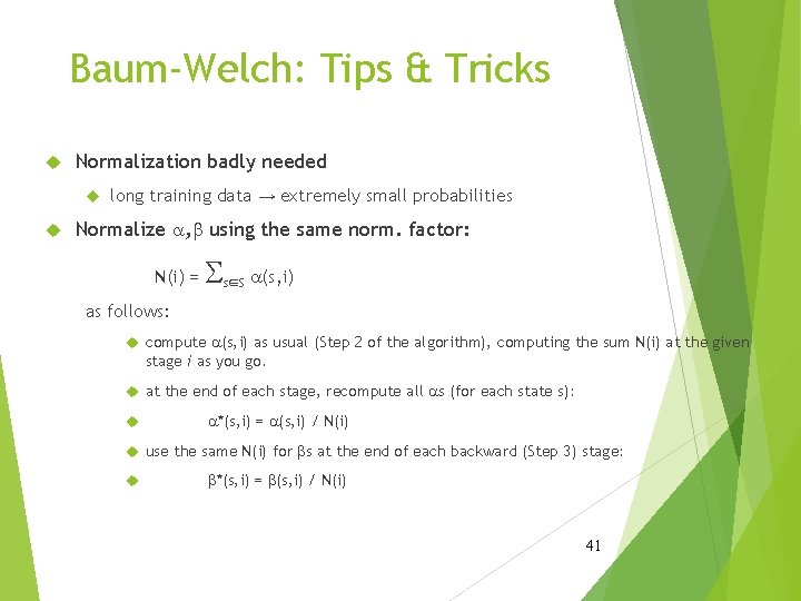
Baum-Welch: Tips & Tricks Normalization badly needed long training data → extremely small probabilities Normalize a, b using the same norm. factor: N(i) = S s∈S a(s, i) as follows: compute a(s, i) as usual (Step 2 of the algorithm), computing the sum N(i) at the given stage i as you go. at the end of each stage, recompute all as (for each state s): a*(s, i) = a(s, i) / N(i) use the same N(i) for bs at the end of each backward (Step 3) stage: b*(s, i) = b(s, i) / N(i) 41
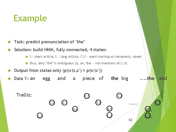
Example Task: predict pronunciation of “the” Solution: build HMM, fully connected, 4 states: S - short article, L - long article, C, V - word starting w/consonant, vowel thus, only “the” is ambiguous (a, an, the - not members of C, V) Output from states only (p(w|s, s’) = p(w|s’)) Data Y: an egg and a Trellis: piece of the big C, 8 C, 5 V, 2 S, 4 L, 1 . . . . V, 6 V, 3 . . the end S, 7 V, T S, T-1 L, 7 42 L, T-1
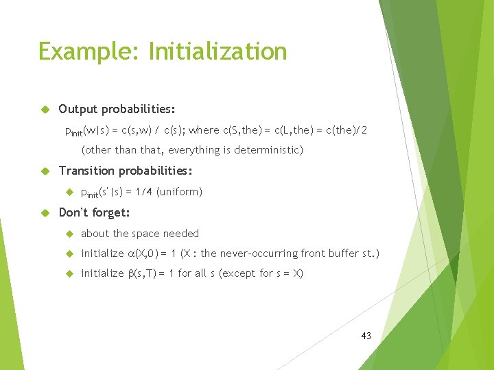
Example: Initialization Output probabilities: pinit(w|s) = c(s, w) / c(s); where c(S, the) = c(L, the) = c(the)/2 (other than that, everything is deterministic) Transition probabilities: pinit(s’|s) = 1/4 (uniform) Don’t forget: about the space needed initialize a(X, 0) = 1 (X : the never-occurring front buffer st. ) initialize b(s, T) = 1 for all s (except for s = X) 43
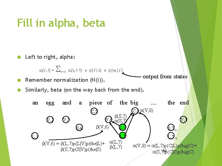
Fill in alpha, beta Left to right, alpha: a(s’, i) = S s→s’ a(s, i-1) ⅹ p(s’|s) ⅹ p(wi|s’) output from states Remember normalization (N(i)). Similarly, beta (on the way back from the end). an egg and a piece of C, 5 V, 2 b(S, 7) . . the end C, 8 a(V, 8) V, 6 a(S, 7) V, 3 S, 4 L, 1 the big b(V, 6) V, T S, 7 S, T-1 L, 7 L, T-1 b(V, 6) = b(L, 7)p(L|V)p(the|L)+ a(L, 7) b(S, 7)p(S|V)p(the|S) a(V, 8) = a(L, 7)p(C|L)p(big|C)+ 44 a(S, 7)p(C|S)p(big|C)
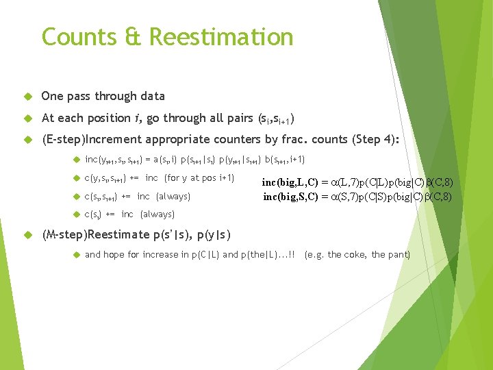
Counts & Reestimation One pass through data At each position i, go through all pairs (si, si+1) (E-step)Increment appropriate counters by frac. counts (Step 4): inc(yi+1, si+1) = a(si, i) p(si+1|si) p(yi+1|si+1) b(si+1, i+1) c(y, si+1) += inc (for y at pos i+1) c(si, si+1) += inc (always) inc(big, L, C) = a(L, 7)p(C|L)p(big|C)b(C, 8) inc(big, S, C) = a(S, 7)p(C|S)p(big|C)b(C, 8) c(si) += inc (always) (M-step)Reestimate p(s’|s), p(y|s) and hope for increase in p(C|L) and p(the|L). . . !! (e. g. the coke, the pant)
HMM: Final Remarks Parameter “tying”: keep certain parameters same (~ just one “counter” for all of them) – data sparseness any combination in principle possible ex. : smoothing (just one set of lambdas) Real Numbers Output Y of infinite size (R, Rn): parametric (typically: few) distribution needed (e. g. , “Gaussian”) “Empty” transitions: do not generate output ~ vertical arcs in trellis; do not use in “counting” 46
- Slides: 46