Market Structure and Competition Copyright c2014 John Wiley

Market Structure and Competition Copyright (c)2014 John Wiley & Sons, Inc. Chapter 13 1

Chapter Thirteen Overview 1. Introduction: Cola Wars 2. A Taxonomy of Market Structures 4. Oligopoly – Interdependence of Strategic Decisions • Bertrand with Homogeneous and Differentiated Products 5. The Effect of a Change in the Strategic Variable • • Theory vs. Observation Cournot Equilibrium (homogeneous) Comparison to Bertrand, Monopoly Reconciling Bertrand, and Cournot 6. The Effect of a Change in Timing: Stackelberg Equilibrium Chapter Thirteen Copyright (c)2014 John Wiley & Sons, Inc. 3. Monopolistic Competition 2

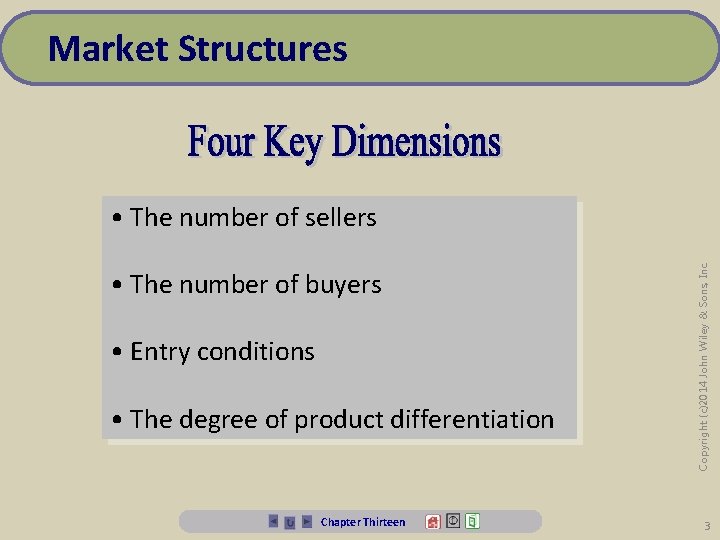
Market Structures • The number of buyers • Entry conditions • The degree of product differentiation Chapter Thirteen Copyright (c)2014 John Wiley & Sons, Inc. • The number of sellers 3

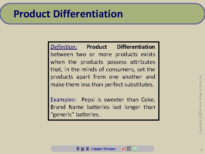
Definition: Product Differentiation between two or more products exists when the products possess attributes that, in the minds of consumers, set the products apart from one another and make them less than perfect substitutes. Examples: Pepsi is sweeter than Coke, Brand Name batteries last longer than "generic" batteries. Chapter Thirteen Copyright (c)2014 John Wiley & Sons, Inc. Product Differentiation 4

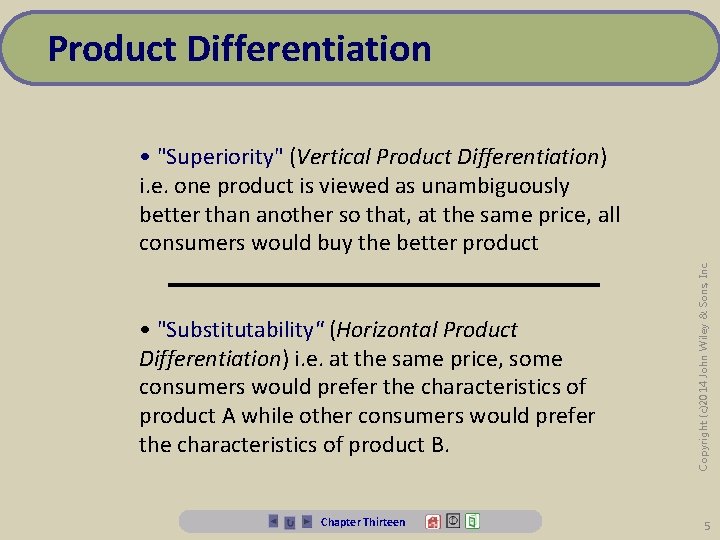
Product Differentiation • "Substitutability" (Horizontal Product Differentiation) i. e. at the same price, some consumers would prefer the characteristics of product A while other consumers would prefer the characteristics of product B. Chapter Thirteen Copyright (c)2014 John Wiley & Sons, Inc. • "Superiority" (Vertical Product Differentiation) i. e. one product is viewed as unambiguously better than another so that, at the same price, all consumers would buy the better product 5

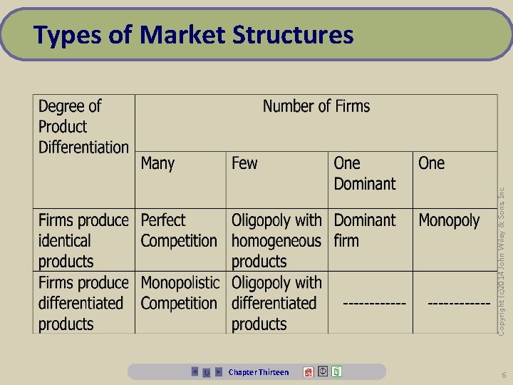
Copyright (c)2014 John Wiley & Sons, Inc. Types of Market Structures Chapter Thirteen 6

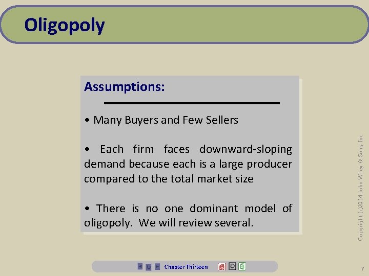
Oligopoly Assumptions: • Each firm faces downward-sloping demand because each is a large producer compared to the total market size • There is no one dominant model of oligopoly. We will review several. Chapter Thirteen Copyright (c)2014 John Wiley & Sons, Inc. • Many Buyers and Few Sellers 7

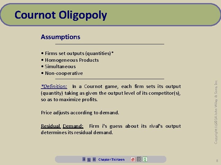
Cournot Oligopoly Assumptions *Definition: In a Cournot game, each firm sets its output (quantity) taking as given the output level of its competitor(s), so as to maximize profits. Price adjusts according to demand. Residual Demand: Firm i's guess about its rival's output determines its residual demand. Chapter Thirteen Copyright (c)2014 John Wiley & Sons, Inc. • Firms set outputs (quantities)* • Homogeneous Products • Simultaneous • Non-cooperative 8

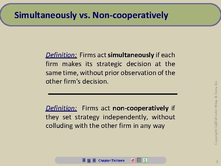
Definition: Firms act simultaneously if each firm makes its strategic decision at the same time, without prior observation of the other firm's decision. Definition: Firms act non-cooperatively if they set strategy independently, without colluding with the other firm in any way Chapter Thirteen Copyright (c)2014 John Wiley & Sons, Inc. Simultaneously vs. Non-cooperatively 9

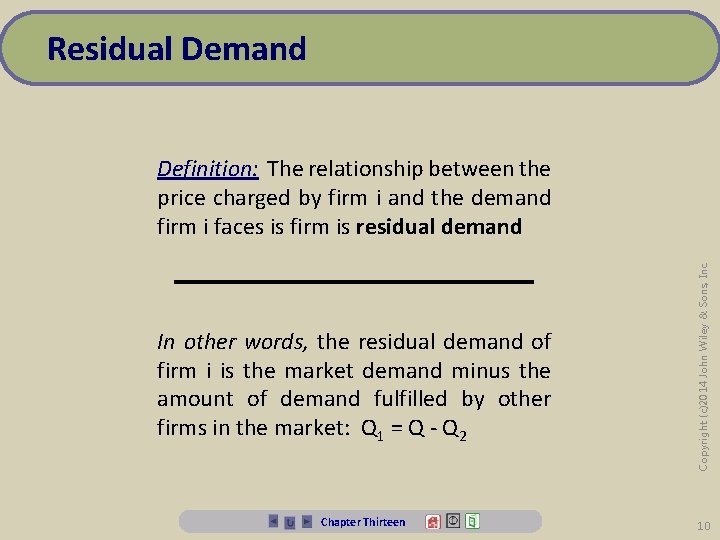
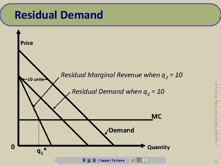
Residual Demand In other words, the residual demand of firm i is the market demand minus the amount of demand fulfilled by other firms in the market: Q 1 = Q - Q 2 Chapter Thirteen Copyright (c)2014 John Wiley & Sons, Inc. Definition: The relationship between the price charged by firm i and the demand firm i faces is firm is residual demand 10

Residual Demand 10 units Residual Marginal Revenue when q 2 = 10 Residual Demand when q 2 = 10 MC Demand 0 Quantity q 1* Chapter Thirteen Copyright (c)2014 John Wiley & Sons, Inc. Price 11

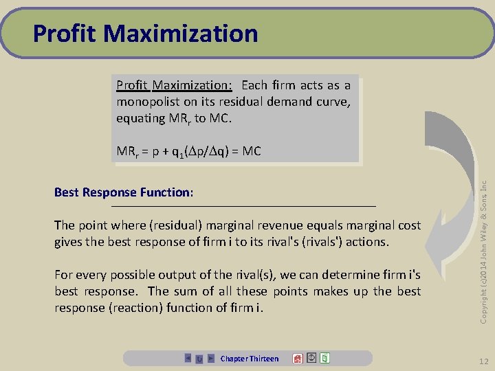
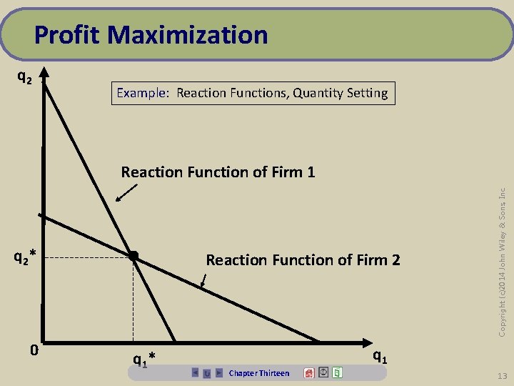
Profit Maximization: Each firm acts as a monopolist on its residual demand curve, equating MRr to MC. Best Response Function: The point where (residual) marginal revenue equals marginal cost gives the best response of firm i to its rival's (rivals') actions. For every possible output of the rival(s), we can determine firm i's best response. The sum of all these points makes up the best response (reaction) function of firm i. Chapter Thirteen Copyright (c)2014 John Wiley & Sons, Inc. MRr = p + q 1( p/ q) = MC 12

Profit Maximization q 2 Example: Reaction Functions, Quantity Setting q 2* 0 • q 1* Reaction Function of Firm 2 Copyright (c)2014 John Wiley & Sons, Inc. Reaction Function of Firm 1 q 1 Chapter Thirteen 13

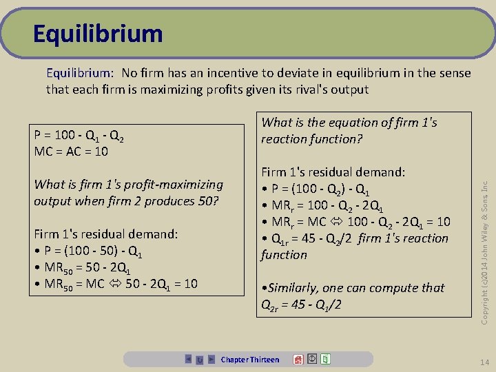
Equilibrium: No firm has an incentive to deviate in equilibrium in the sense that each firm is maximizing profits given its rival's output P = 100 - Q 1 - Q 2 MC = AC = 10 What is firm 1's profit-maximizing output when firm 2 produces 50? Firm 1's residual demand: • P = (100 - 50) - Q 1 • MR 50 = 50 - 2 Q 1 • MR 50 = MC 50 - 2 Q 1 = 10 Firm 1's residual demand: • P = (100 - Q 2) - Q 1 • MRr = 100 - Q 2 - 2 Q 1 • MRr = MC 100 - Q 2 - 2 Q 1 = 10 • Q 1 r = 45 - Q 2/2 firm 1's reaction function • Similarly, one can compute that Q 2 r = 45 - Q 1/2 Chapter Thirteen Copyright (c)2014 John Wiley & Sons, Inc. What is the equation of firm 1's reaction function? 14

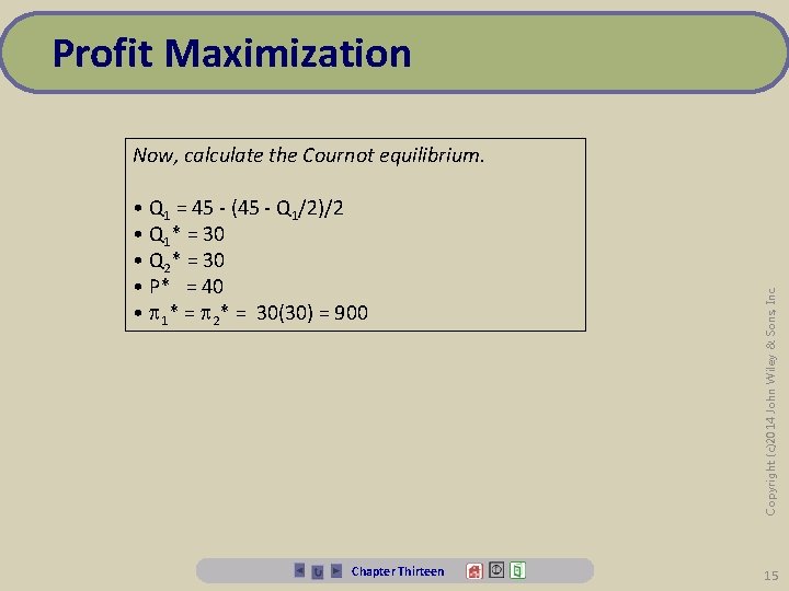
Profit Maximization • Q 1 = 45 - (45 - Q 1/2)/2 • Q 1* = 30 • Q 2* = 30 • P* = 40 • 1* = 2* = 30(30) = 900 Chapter Thirteen Copyright (c)2014 John Wiley & Sons, Inc. Now, calculate the Cournot equilibrium. 15

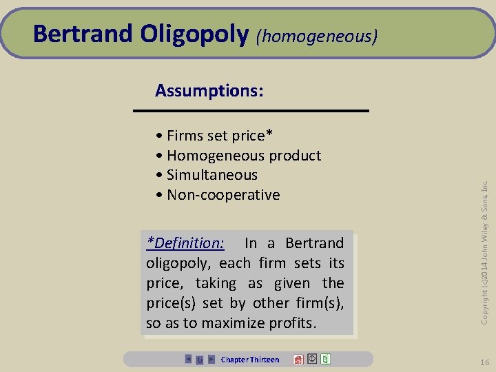
Bertrand Oligopoly (homogeneous) • Firms set price* • Homogeneous product • Simultaneous • Non-cooperative *Definition: In a Bertrand oligopoly, each firm sets its price, taking as given the price(s) set by other firm(s), so as to maximize profits. Chapter Thirteen Copyright (c)2014 John Wiley & Sons, Inc. Assumptions: 16

Setting Price • Further, each firm realizes that the demand that it faces depends both on its own price and on the price set by other firms • Specifically, any firm charging a higher price than its rivals will sell no output. • Any firm charging a lower price than its rivals will obtain the entire market demand. Chapter Thirteen Copyright (c)2014 John Wiley & Sons, Inc. • Homogeneity implies that consumers will buy from the low-price seller. 17

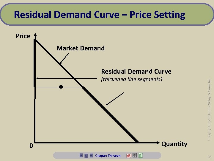
Residual Demand Curve – Price Setting Price Market Demand • (thickened line segments) Quantity 0 Chapter Thirteen Copyright (c)2014 John Wiley & Sons, Inc. Residual Demand Curve 18

• Assume firm always meets its residual demand (no capacity constraints) • Assume that marginal cost is constant at c per unit. • Hence, any price at least equal to c ensures nonnegative profits. Chapter Thirteen Copyright (c)2014 John Wiley & Sons, Inc. Residual Demand Curve – Price Setting 19

Best Response Function Definition: The firm's profit maximizing action as a function of the action by the rival firm is the firm's best response (or reaction) function Example: 2 firms Bertrand competitors Firm 1's best response function is P 1=P 2 - e Firm 2's best response function is P 2=P 1 - e Chapter Thirteen Copyright (c)2014 John Wiley & Sons, Inc. Each firm's profit maximizing response to the other firm's price is to undercut (as long as P > MC) 20

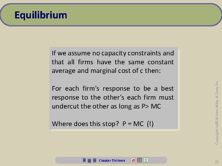
Equilibrium For each firm's response to be a best response to the other's each firm must undercut the other as long as P> MC Where does this stop? P = MC (!) Chapter Thirteen Copyright (c)2014 John Wiley & Sons, Inc. If we assume no capacity constraints and that all firms have the same constant average and marginal cost of c then: 21

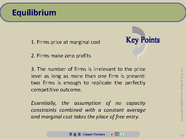
Equilibrium 1. Firms price at marginal cost 3. The number of firms is irrelevant to the price level as long as more than one firm is present: two firms is enough to replicate the perfectly competitive outcome. Essentially, the assumption of no capacity constraints combined with a constant average and marginal cost takes the place of free entry. Chapter Thirteen Copyright (c)2014 John Wiley & Sons, Inc. 2. Firms make zero profits 22

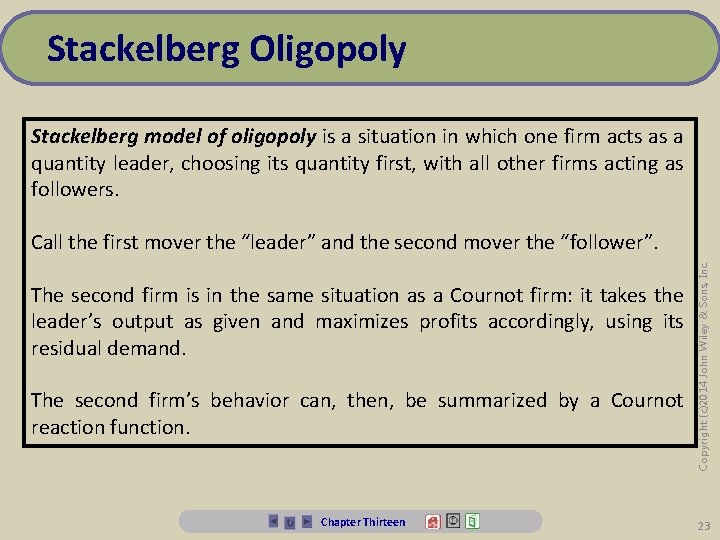
Stackelberg Oligopoly Stackelberg model of oligopoly is a situation in which one firm acts as a quantity leader, choosing its quantity first, with all other firms acting as followers. The second firm is in the same situation as a Cournot firm: it takes the leader’s output as given and maximizes profits accordingly, using its residual demand. The second firm’s behavior can, then, be summarized by a Cournot reaction function. Chapter Thirteen Copyright (c)2014 John Wiley & Sons, Inc. Call the first mover the “leader” and the second mover the “follower”. 23

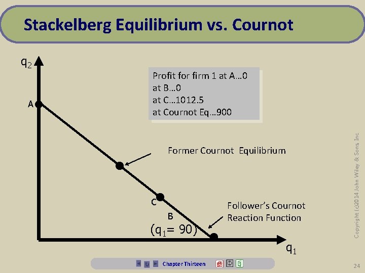
Stackelberg Equilibrium vs. Cournot q 2 • Former Cournot Equilibrium • • C B (q 1= 90) Chapter Thirteen • Follower’s Cournot Reaction Function Copyright (c)2014 John Wiley & Sons, Inc. A Profit for firm 1 at A… 0 at B… 0 at C… 1012. 5 at Cournot Eq… 900 q 1 24

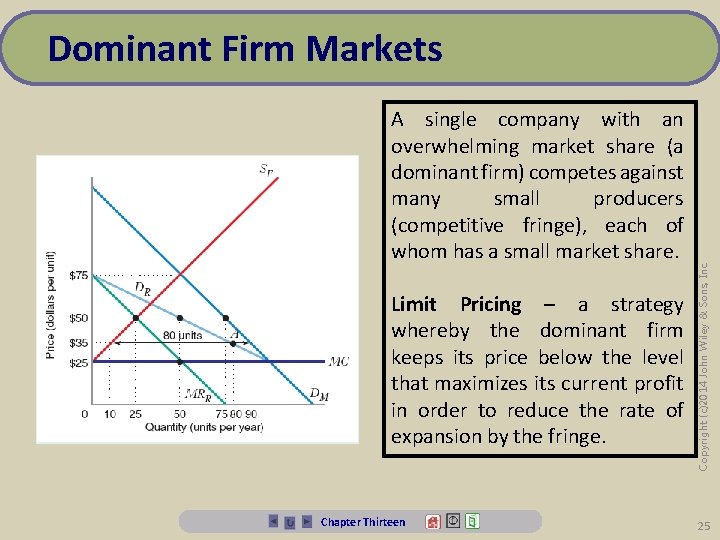
A single company with an overwhelming market share (a dominant firm) competes against many small producers (competitive fringe), each of whom has a small market share. Limit Pricing – a strategy whereby the dominant firm keeps its price below the level that maximizes its current profit in order to reduce the rate of expansion by the fringe. Chapter Thirteen Copyright (c)2014 John Wiley & Sons, Inc. Dominant Firm Markets 25

Bertrand Competition – Differentiated Firms set price* Differentiated product Simultaneous Non-cooperative *Differentiation means that lowering price below your rivals' will not result in capturing the entire market, nor will raising price mean losing the entire market so that residual demand decreases smoothly Chapter Thirteen Copyright (c)2014 John Wiley & Sons, Inc. Assumptions: 26

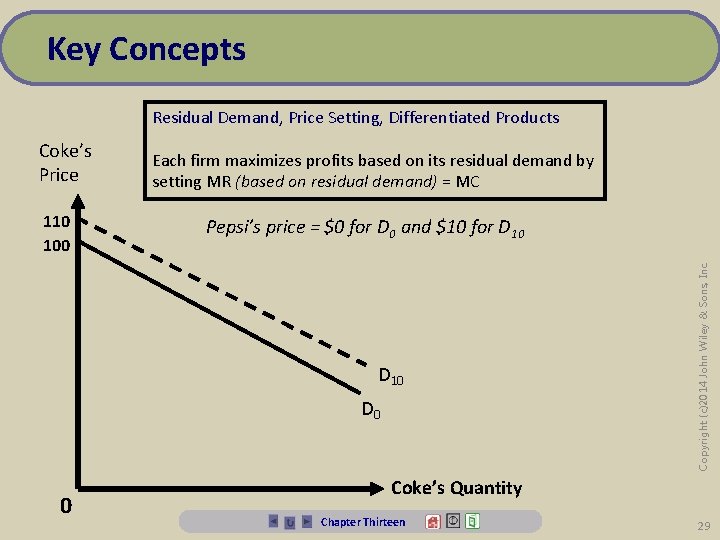
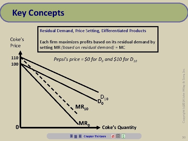
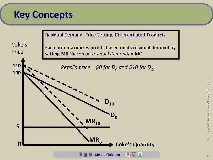
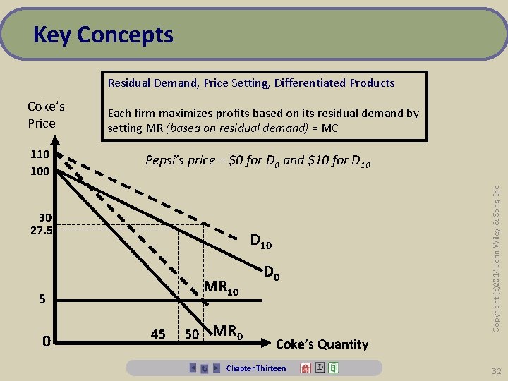
Bertrand Competition – Differentiated MC 1 = MC 2 = 5 What is firm 1's residual demand when Firm 2's price is $10? $0? Q 1(10) = 100 - 2 P 1 + 10 = 110 - 2 P 1 Q 1(0) = 100 - 2 P 1 + 0 = 100 - 2 P 1 Chapter Thirteen Copyright (c)2014 John Wiley & Sons, Inc. Q 1 = 100 - 2 P 1 + P 2 "Coke's demand" Q 2 = 100 - 2 P 2 + P 1 "Pepsi's demand" 27

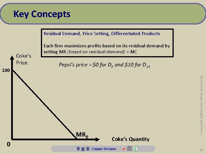
Key Concepts Residual Demand, Price Setting, Differentiated Products 100 Pepsi’s price = $0 for D 0 and $10 for D 10 MR 0 0 Copyright (c)2014 John Wiley & Sons, Inc. Coke’s Price Each firm maximizes profits based on its residual demand by setting MR (based on residual demand) = MC Coke’s Quantity Chapter Thirteen 28

Key Concepts Residual Demand, Price Setting, Differentiated Products 110 100 Each firm maximizes profits based on its residual demand by setting MR (based on residual demand) = MC Pepsi’s price = $0 for D 0 and $10 for D 10 D 0 0 Copyright (c)2014 John Wiley & Sons, Inc. Coke’s Price Coke’s Quantity Chapter Thirteen 29

Key Concepts Residual Demand, Price Setting, Differentiated Products 110 100 Each firm maximizes profits based on its residual demand by setting MR (based on residual demand) = MC Pepsi’s price = $0 for D 0 and $10 for D 10 MR 10 0 MR 0 D 10 D 0 Copyright (c)2014 John Wiley & Sons, Inc. Coke’s Price Coke’s Quantity Chapter Thirteen 30

Key Concepts Residual Demand, Price Setting, Differentiated Products 110 100 Each firm maximizes profits based on its residual demand by setting MR (based on residual demand) = MC Pepsi’s price = $0 for D 0 and $10 for D 10 5 0 MR 10 MR 0 D 0 Copyright (c)2014 John Wiley & Sons, Inc. Coke’s Price Coke’s Quantity Chapter Thirteen 31

Key Concepts Residual Demand, Price Setting, Differentiated Products 110 100 Each firm maximizes profits based on its residual demand by setting MR (based on residual demand) = MC Pepsi’s price = $0 for D 0 and $10 for D 10 30 27. 5 D 10 MR 10 5 0 45 50 MR 0 D 0 Copyright (c)2014 John Wiley & Sons, Inc. Coke’s Price Coke’s Quantity Chapter Thirteen 32

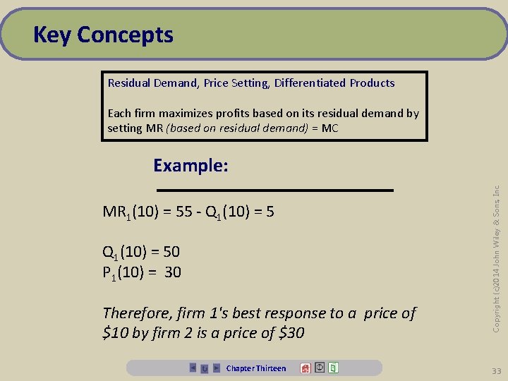
Key Concepts Residual Demand, Price Setting, Differentiated Products Each firm maximizes profits based on its residual demand by setting MR (based on residual demand) = MC MR 1(10) = 55 - Q 1(10) = 50 P 1(10) = 30 Therefore, firm 1's best response to a price of $10 by firm 2 is a price of $30 Chapter Thirteen Copyright (c)2014 John Wiley & Sons, Inc. Example: 33

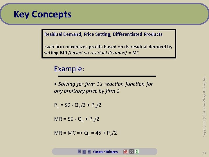
Key Concepts Residual Demand, Price Setting, Differentiated Products Each firm maximizes profits based on its residual demand by setting MR (based on residual demand) = MC MR = MC => Q 1 = 45 + P 2/2 Copyright (c)2014 John Wiley & Sons, Inc. Example: Chapter Thirteen 34 • Solving for firm 1's reaction function for any arbitrary price by firm 2 P 1 = 50 - Q 1/2 + P 2/2 MR = 50 - Q 1 + P 2/2

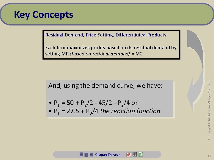
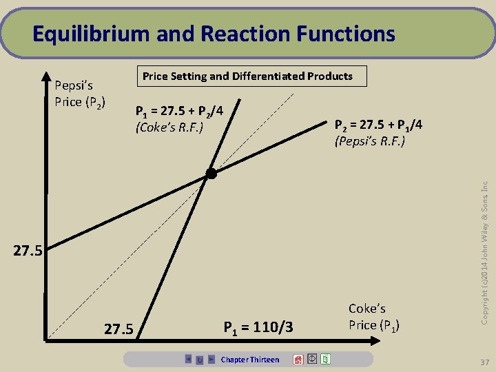
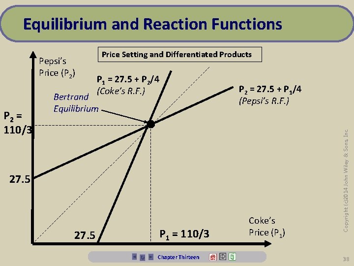
Key Concepts Residual Demand, Price Setting, Differentiated Products And, using the demand curve, we have: • P 1 = 50 + P 2/2 - 45/2 - P 2/4 or • P 1 = 27. 5 + P 2/4 the reaction function Chapter Thirteen Copyright (c)2014 John Wiley & Sons, Inc. Each firm maximizes profits based on its residual demand by setting MR (based on residual demand) = MC 35

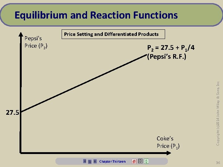
Equilibrium and Reaction Functions Price Setting and Differentiated Products P 2 = 27. 5 + P 1/4 (Pepsi’s R. F. ) 27. 5 Coke’s Price (P 1) Chapter Thirteen Copyright (c)2014 John Wiley & Sons, Inc. Pepsi’s Price (P 2) 36

Equilibrium and Reaction Functions Price Setting and Differentiated Products P 1 = 27. 5 + P 2/4 (Coke’s R. F. ) P 2 = 27. 5 + P 1/4 (Pepsi’s R. F. ) • 27. 5 P 1 = 110/3 Chapter Thirteen Coke’s Price (P 1) Copyright (c)2014 John Wiley & Sons, Inc. Pepsi’s Price (P 2) 37

Equilibrium and Reaction Functions P 2 = 110/3 Price Setting and Differentiated Products P 1 = 27. 5 + P 2/4 (Coke’s R. F. ) Bertrand Equilibrium P 2 = 27. 5 + P 1/4 (Pepsi’s R. F. ) • 27. 5 P 1 = 110/3 Chapter Thirteen Coke’s Price (P 1) Copyright (c)2014 John Wiley & Sons, Inc. Pepsi’s Price (P 2) 38

Equilibrium occurs when all firms simultaneously choose their best response to each others' actions. Graphically, this amounts to the point where the best response functions cross. Chapter Thirteen Copyright (c)2014 John Wiley & Sons, Inc. Equilibrium 39

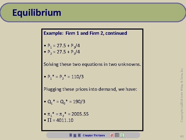
Equilibrium Example: Firm 1 and Firm 2, continued • P 1 = 27. 5 + P 2/4 • P 2 = 27. 5 + P 1/4 • P 1* = P 2* = 110/3 Plugging these prices into demand, we have: • Q 1* = Q 2* = 190/3 • 1* = 2005. 55 • = 4011. 10 Chapter Thirteen Copyright (c)2014 John Wiley & Sons, Inc. Solving these two equations in two unknowns. 40

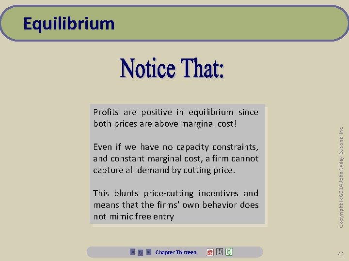
Profits are positive in equilibrium since both prices are above marginal cost! Even if we have no capacity constraints, and constant marginal cost, a firm cannot capture all demand by cutting price. This blunts price-cutting incentives and means that the firms' own behavior does not mimic free entry Chapter Thirteen Copyright (c)2014 John Wiley & Sons, Inc. Equilibrium 41

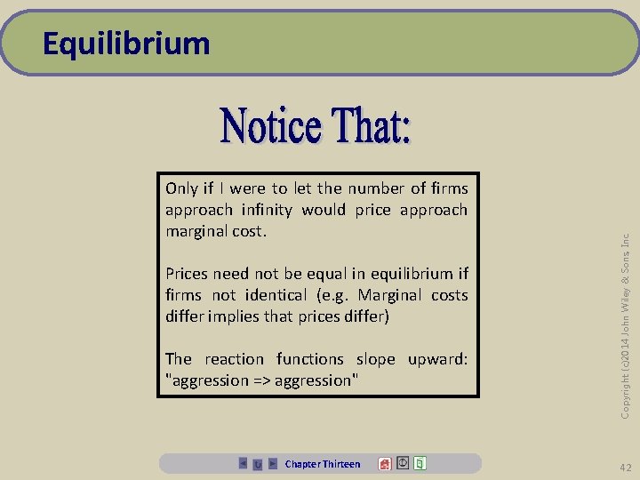
Only if I were to let the number of firms approach infinity would price approach marginal cost. Prices need not be equal in equilibrium if firms not identical (e. g. Marginal costs differ implies that prices differ) The reaction functions slope upward: "aggression => aggression" Chapter Thirteen Copyright (c)2014 John Wiley & Sons, Inc. Equilibrium 42

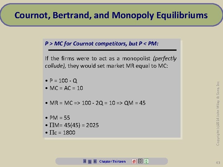
Cournot, Bertrand, and Monopoly Equilibriums P > MC for Cournot competitors, but P < PM: • P = 100 - Q • MC = AC = 10 • MR = MC => 100 - 2 Q = 10 => QM = 45 • PM = 55 • M= 45(45) = 2025 • c = 1800 Chapter Thirteen Copyright (c)2014 John Wiley & Sons, Inc. If the firms were to act as a monopolist (perfectly collude), they would set market MR equal to MC: 43

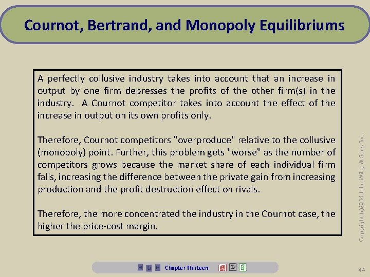
Cournot, Bertrand, and Monopoly Equilibriums Therefore, Cournot competitors "overproduce" relative to the collusive (monopoly) point. Further, this problem gets "worse" as the number of competitors grows because the market share of each individual firm falls, increasing the difference between the private gain from increasing production and the profit destruction effect on rivals. Therefore, the more concentrated the industry in the Cournot case, the higher the price-cost margin. Chapter Thirteen Copyright (c)2014 John Wiley & Sons, Inc. A perfectly collusive industry takes into account that an increase in output by one firm depresses the profits of the other firm(s) in the industry. A Cournot competitor takes into account the effect of the increase in output on its own profits only. 44

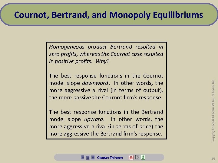
Cournot, Bertrand, and Monopoly Equilibriums The best response functions in the Cournot model slope downward. In other words, the more aggressive a rival (in terms of output), the more passive the Cournot firm's response. The best response functions in the Bertrand model slope upward. In other words, the more aggressive a rival (in terms of price) the more aggressive the Bertrand firm's response. Chapter Thirteen Copyright (c)2014 John Wiley & Sons, Inc. Homogeneous product Bertrand resulted in zero profits, whereas the Cournot case resulted in positive profits. Why? 45

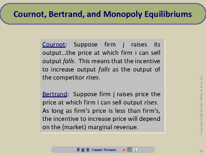
Cournot: Suppose firm j raises its output…the price at which firm i can sell output falls. This means that the incentive to increase output falls as the output of the competitor rises. Bertrand: Suppose firm j raises price the price at which firm i can sell output rises. As long as firm's price is less than firm's, the incentive to increase price will depend on the (market) marginal revenue. Chapter Thirteen Copyright (c)2014 John Wiley & Sons, Inc. Cournot, Bertrand, and Monopoly Equilibriums 46

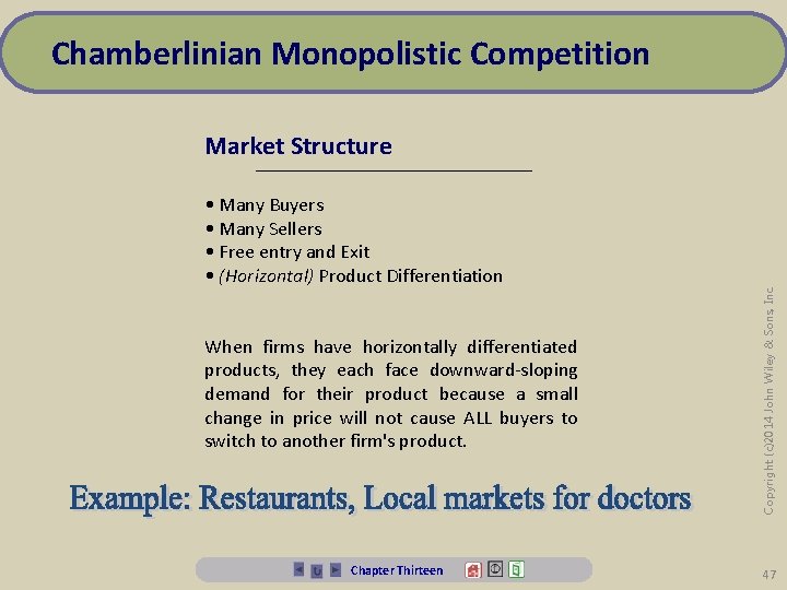
Chamberlinian Monopolistic Competition • Many Buyers • Many Sellers • Free entry and Exit • (Horizontal) Product Differentiation When firms have horizontally differentiated products, they each face downward-sloping demand for their product because a small change in price will not cause ALL buyers to switch to another firm's product. Chapter Thirteen Copyright (c)2014 John Wiley & Sons, Inc. Market Structure 47

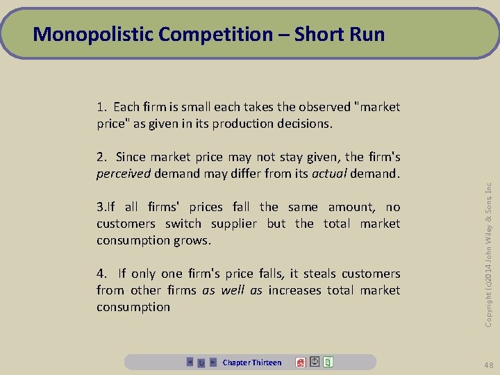
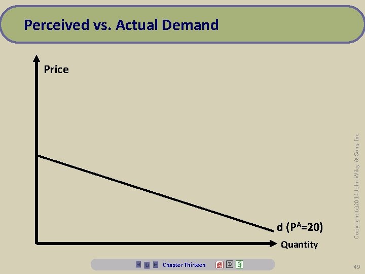
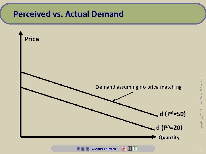
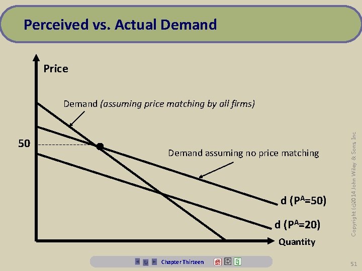
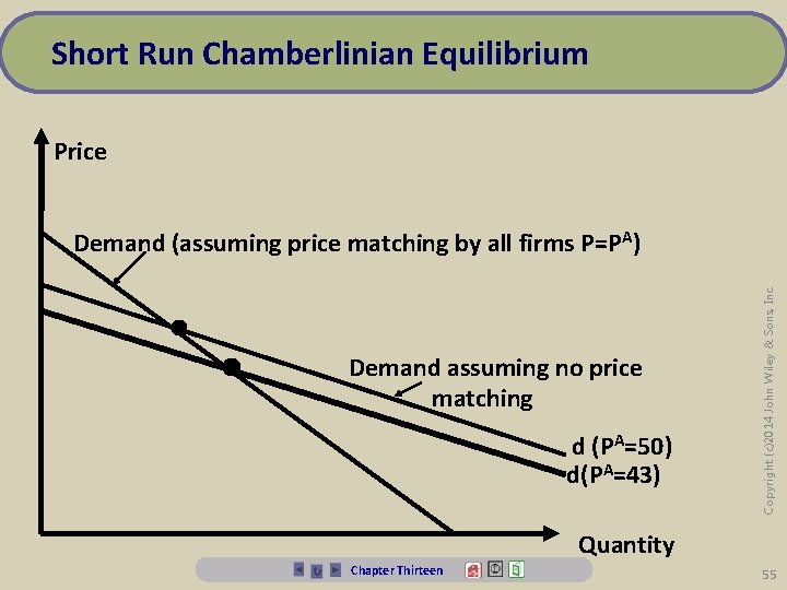
Monopolistic Competition – Short Run 2. Since market price may not stay given, the firm's perceived demand may differ from its actual demand. 3. If all firms' prices fall the same amount, no customers switch supplier but the total market consumption grows. 4. If only one firm's price falls, it steals customers from other firms as well as increases total market consumption Chapter Thirteen Copyright (c)2014 John Wiley & Sons, Inc. 1. Each firm is small each takes the observed "market price" as given in its production decisions. 48

Perceived vs. Actual Demand d (PA=20) Quantity Chapter Thirteen Copyright (c)2014 John Wiley & Sons, Inc. Price 49

Perceived vs. Actual Demand assuming no price matching d (PA=50) d (PA=20) Quantity Chapter Thirteen Copyright (c)2014 John Wiley & Sons, Inc. Price 50

Perceived vs. Actual Demand Price 50 • Demand assuming no price matching d (PA=50) d (PA=20) Quantity Chapter Thirteen Copyright (c)2014 John Wiley & Sons, Inc. Demand (assuming price matching by all firms) 51

Market Equilibrium • Each firm maximizes profit taking the average market price as given • Each firm can sell the quantity it desires at the actual average market price that prevails Chapter Thirteen Copyright (c)2014 John Wiley & Sons, Inc. The market is in equilibrium if: 52

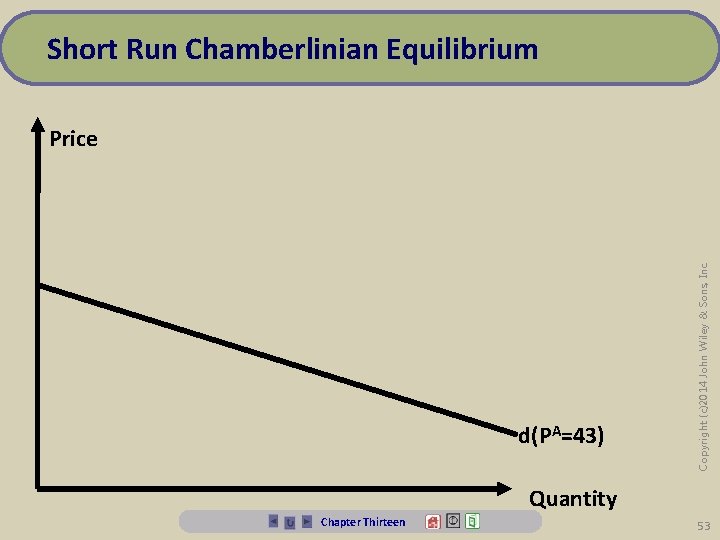
Short Run Chamberlinian Equilibrium d(PA=43) Copyright (c)2014 John Wiley & Sons, Inc. Price Quantity Chapter Thirteen 53

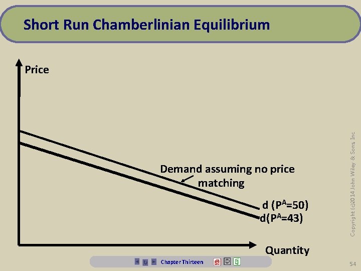
Short Run Chamberlinian Equilibrium Demand assuming no price matching d (PA=50) d(PA=43) Copyright (c)2014 John Wiley & Sons, Inc. Price Quantity Chapter Thirteen 54

Short Run Chamberlinian Equilibrium Price • • Demand assuming no price matching d (PA=50) d(PA=43) Copyright (c)2014 John Wiley & Sons, Inc. Demand (assuming price matching by all firms P=PA) Quantity Chapter Thirteen 55

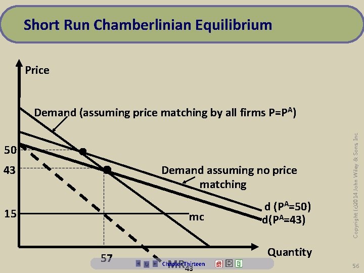
Short Run Chamberlinian Equilibrium Price 50 43 • • 15 Demand assuming no price matching mc 57 MR 43 Chapter Thirteen d (PA=50) d(PA=43) Copyright (c)2014 John Wiley & Sons, Inc. Demand (assuming price matching by all firms P=PA) Quantity 56

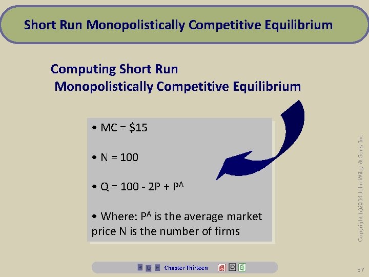
Short Run Monopolistically Competitive Equilibrium • MC = $15 • N = 100 • Q = 100 - 2 P + PA • Where: PA is the average market price N is the number of firms Chapter Thirteen Copyright (c)2014 John Wiley & Sons, Inc. Computing Short Run Monopolistically Competitive Equilibrium 57

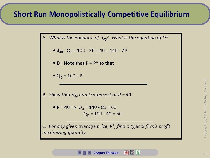
Short Run Monopolistically Competitive Equilibrium A. What is the equation of d 40? What is the equation of D? • d 40: Qd = 100 - 2 P + 40 = 140 - 2 P • QD = 100 - P B. Show that d 40 and D intersect at P = 40 • P = 40 => Qd = 140 - 80 = 60 QD = 100 - 40 = 60 C. For any given average price, PA, find a typical firm's profit maximizing quantity Chapter Thirteen Copyright (c)2014 John Wiley & Sons, Inc. • D: Note that P = PA so that 58

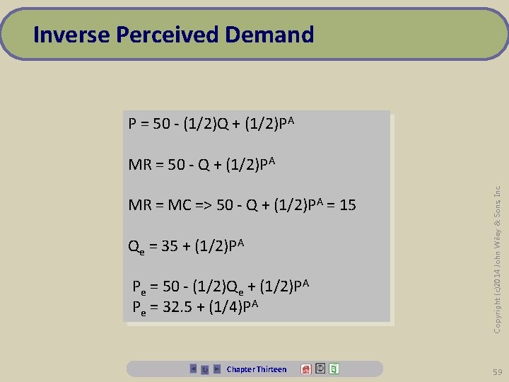
Inverse Perceived Demand P = 50 - (1/2)Q + (1/2)PA MR = MC => 50 - Q + (1/2)PA = 15 Qe = 35 + (1/2)PA Pe = 50 - (1/2)Qe + (1/2)PA Pe = 32. 5 + (1/4)PA Chapter Thirteen Copyright (c)2014 John Wiley & Sons, Inc. MR = 50 - Q + (1/2)PA 59

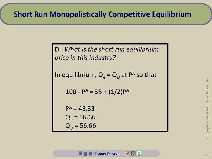
Short Run Monopolistically Competitive Equilibrium In equilibrium, Qe = QD at PA so that 100 - PA = 35 + (1/2)PA PA = 43. 33 Qe = 56. 66 QD = 56. 66 Chapter Thirteen Copyright (c)2014 John Wiley & Sons, Inc. D. What is the short run equilibrium price in this industry? 60

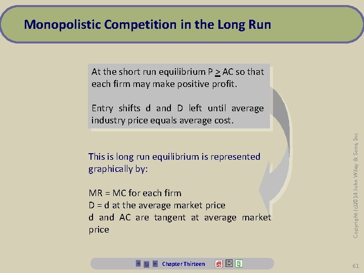
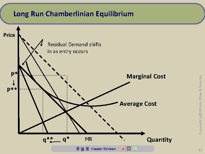
Monopolistic Competition in the Long Run At the short run equilibrium P > AC so that each firm may make positive profit. This is long run equilibrium is represented graphically by: MR = MC for each firm D = d at the average market price d and AC are tangent at average market price Chapter Thirteen Copyright (c)2014 John Wiley & Sons, Inc. Entry shifts d and D left until average industry price equals average cost. 61

Long Run Chamberlinian Equilibrium Price P* Marginal Cost P** Average Cost q** q* MR Chapter Thirteen Copyright (c)2014 John Wiley & Sons, Inc. Residual Demand shifts in as entry occurs Quantity 62

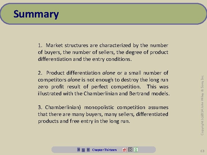
Summary 2. Product differentiation alone or a small number of competitors alone is not enough to destroy the long run zero profit result of perfect competition. This was illustrated with the Chamberlinian and Bertrand models. 3. Chamberlinian) monopolistic competition assumes that there are many buyers, many sellers, differentiated products and free entry in the long run. Chapter Thirteen Copyright (c)2014 John Wiley & Sons, Inc. 1. Market structures are characterized by the number of buyers, the number of sellers, the degree of product differentiation and the entry conditions. 63

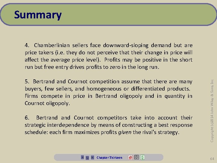
Summary 5. Bertrand Cournot competition assume that there are many buyers, few sellers, and homogeneous or differentiated products. Firms compete in price in Bertrand oligopoly and in quantity in Cournot oligopoly. 6. Bertrand Cournot competitors take into account their strategic interdependence by means of constructing a best response schedule: each firm maximizes profits given the rival's strategy. Chapter Thirteen Copyright (c)2014 John Wiley & Sons, Inc. 4. Chamberlinian sellers face downward-sloping demand but are price takers (i. e. they do not perceive that their change in price will affect the average price level). Profits may be positive in the short run but free entry drives profits to zero in the long run. 64

Summary 8. If the products are homogeneous, the Bertrand equilibrium results in zero profits. By changing the strategic variable from price to quantity, we obtain much higher prices (and profits). Further, the results are sensitive to the assumption of simultaneous moves. 9. This result can be traced to the slope of the reaction functions: upwards in the case of Bertrand downwards in the case of Cournot. These slopes imply that "aggressivity" results in a "passive" response in the Cournot case and an "aggressive" response in the Bertrand case. Chapter Thirteen Copyright (c)2014 John Wiley & Sons, Inc. 7. Equilibrium in such a setting requires that all firms be on their best response functions. 65