Market Risk Va R Model Building Approach Chapter

The Model-Building Approach l l The main alternative to historical simulation is to make assumptions about the probability distributions of the returns on the market variables This is known as the model building approach (or sometimes the variance-covariance approach) Risk Management and Financial Institutions 3 e, Chapter 15, Copyright © John C. Hull 2012 2

Microsoft Example (page 323 -324) l l l We have a position worth $10 million in Microsoft shares The volatility of Microsoft is 2% per day (about 32% per year) We use N=10 and X=99 Risk Management and Financial Institutions 3 e, Chapter 15, Copyright © John C. Hull 2012 3

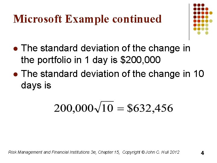
Microsoft Example continued l l The standard deviation of the change in the portfolio in 1 day is $200, 000 The standard deviation of the change in 10 days is Risk Management and Financial Institutions 3 e, Chapter 15, Copyright © John C. Hull 2012 4

Microsoft Example continued l l l We assume that the expected change in the value of the portfolio is zero (This is OK for short time periods) We assume that the change in the value of the portfolio is normally distributed Since N(– 2. 33)=0. 01, the Va. R is Risk Management and Financial Institutions 3 e, Chapter 15, Copyright © John C. Hull 2012 5

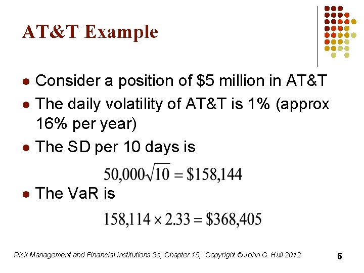
AT&T Example l Consider a position of $5 million in AT&T The daily volatility of AT&T is 1% (approx 16% per year) The SD per 10 days is l The Va. R is l l Risk Management and Financial Institutions 3 e, Chapter 15, Copyright © John C. Hull 2012 6

Portfolio (page 325) l l Now consider a portfolio consisting of both Microsoft and AT&T Suppose that the correlation between the returns is 0. 3 Risk Management and Financial Institutions 3 e, Chapter 15, Copyright © John C. Hull 2012 7

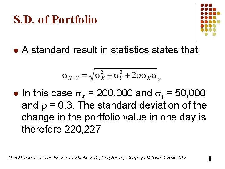
S. D. of Portfolio l l A standard result in statistics states that In this case s. X = 200, 000 and s. Y = 50, 000 and r = 0. 3. The standard deviation of the change in the portfolio value in one day is therefore 220, 227 Risk Management and Financial Institutions 3 e, Chapter 15, Copyright © John C. Hull 2012 8

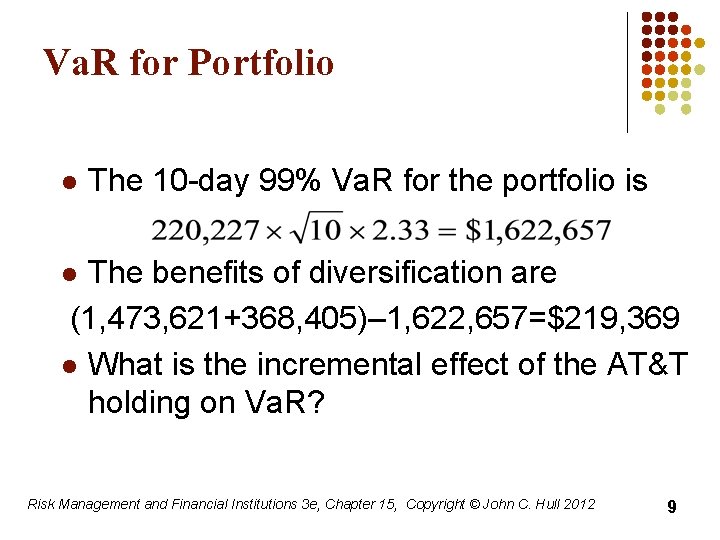
Va. R for Portfolio l The 10 -day 99% Va. R for the portfolio is The benefits of diversification are (1, 473, 621+368, 405)– 1, 622, 657=$219, 369 l What is the incremental effect of the AT&T holding on Va. R? l Risk Management and Financial Institutions 3 e, Chapter 15, Copyright © John C. Hull 2012 9

The Linear Model We assume l The daily change in the value of a portfolio is linearly related to the daily returns from market variables l The returns from the market variables are normally distributed Risk Management and Financial Institutions 3 e, Chapter 15, Copyright © John C. Hull 2012 10

Markowitz Result for Variance of Return on Portfolio Risk Management and Financial Institutions 3

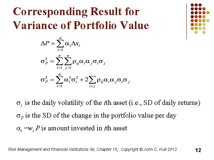
Corresponding Result for Variance of Portfolio Value si is the daily volatility of the ith asset (i. e. , SD of daily returns) s. P is the SD of the change in the portfolio value per day ai =wi P is amount invested in ith asset Risk Management and Financial Institutions 3 e, Chapter 15, Copyright © John C. Hull 2012 12

Covariance Matrix (vari = covii) (page 328) Risk Management and Financial Institutions 3 e,

Alternative Expressions for s. P 2 page 328 Risk Management and Financial Institutions 3

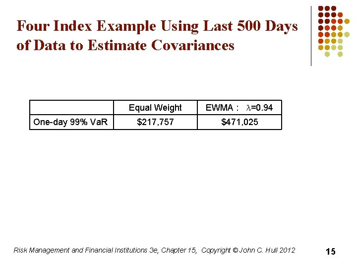
Four Index Example Using Last 500 Days of Data to Estimate Covariances One-day 99% Va. R Equal Weight EWMA : l=0. 94 $217, 757 $471, 025 Risk Management and Financial Institutions 3 e, Chapter 15, Copyright © John C. Hull 2012 15

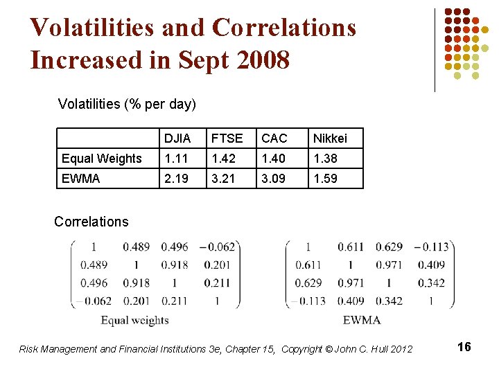
Volatilities and Correlations Increased in Sept 2008 Volatilities (% per day) DJIA FTSE CAC Nikkei Equal Weights 1. 11 1. 42 1. 40 1. 38 EWMA 2. 19 3. 21 3. 09 1. 59 Correlations Risk Management and Financial Institutions 3 e, Chapter 15, Copyright © John C. Hull 2012 16

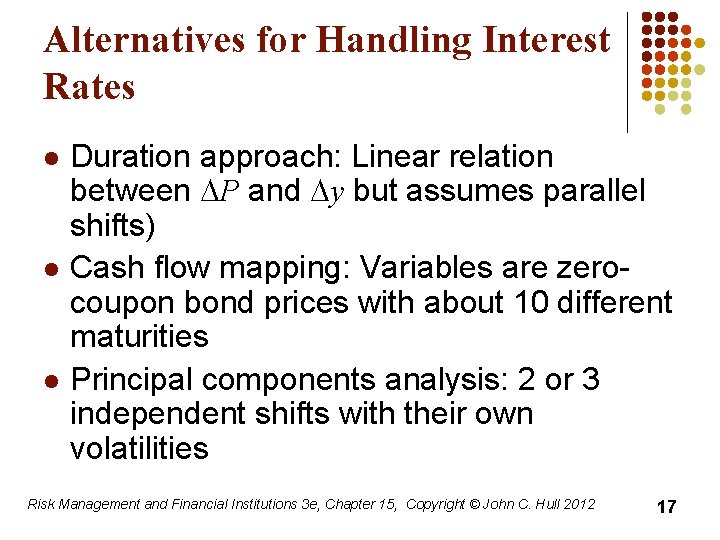
Alternatives for Handling Interest Rates l l l Duration approach: Linear relation between DP and Dy but assumes parallel shifts) Cash flow mapping: Variables are zerocoupon bond prices with about 10 different maturities Principal components analysis: 2 or 3 independent shifts with their own volatilities Risk Management and Financial Institutions 3 e, Chapter 15, Copyright © John C. Hull 2012 17

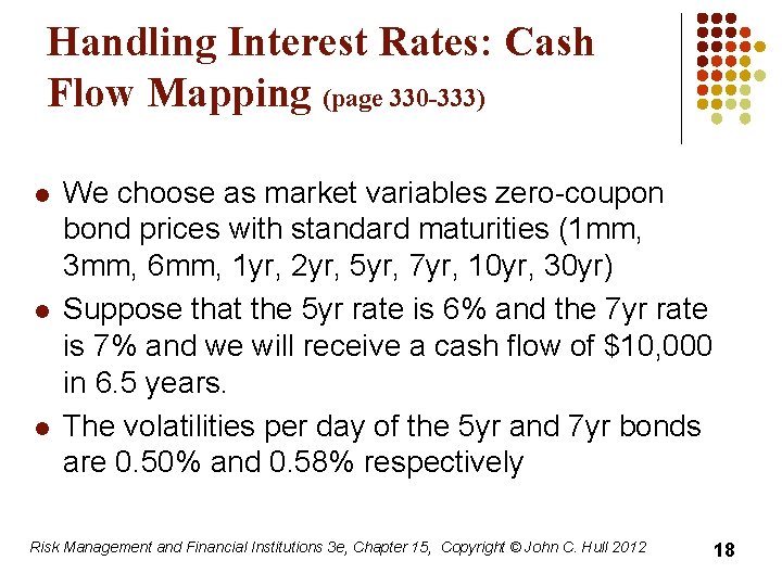
Handling Interest Rates: Cash Flow Mapping (page 330 -333) l l l We choose as market variables zero-coupon bond prices with standard maturities (1 mm, 3 mm, 6 mm, 1 yr, 2 yr, 5 yr, 7 yr, 10 yr, 30 yr) Suppose that the 5 yr rate is 6% and the 7 yr rate is 7% and we will receive a cash flow of $10, 000 in 6. 5 years. The volatilities per day of the 5 yr and 7 yr bonds are 0. 50% and 0. 58% respectively Risk Management and Financial Institutions 3 e, Chapter 15, Copyright © John C. Hull 2012 18

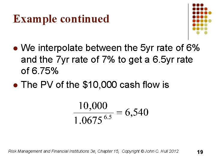
Example continued l l We interpolate between the 5 yr rate of 6% and the 7 yr rate of 7% to get a 6. 5 yr rate of 6. 75% The PV of the $10, 000 cash flow is Risk Management and Financial Institutions 3 e, Chapter 15, Copyright © John C. Hull 2012 19

Example continued l l We interpolate between the 0. 5% volatility for the 5 yr bond price and the 0. 58% volatility for the 7 yr bond price to get 0. 56% as the volatility for the 6. 5 yr bond We allocate a of the PV to the 5 yr bond and (1 - a) of the PV to the 7 yr bond Risk Management and Financial Institutions 3 e, Chapter 15, Copyright © John C. Hull 2012 20

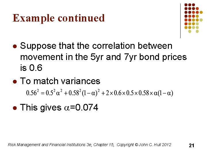
Example continued l Suppose that the correlation between movement in the 5 yr and 7 yr bond prices is 0. 6 To match variances l This gives a=0. 074 l Risk Management and Financial Institutions 3 e, Chapter 15, Copyright © John C. Hull 2012 21

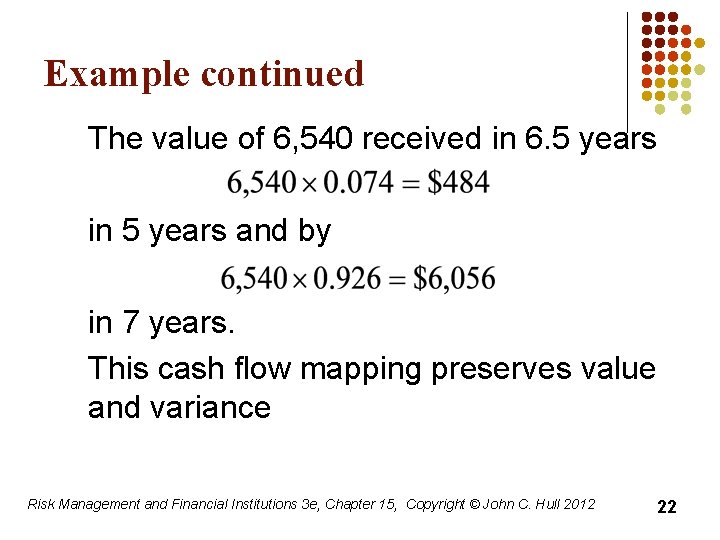
Example continued The value of 6, 540 received in 6. 5 years in 5 years and by in 7 years. This cash flow mapping preserves value and variance Risk Management and Financial Institutions 3 e, Chapter 15, Copyright © John C. Hull 2012 22

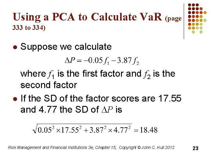
Using a PCA to Calculate Va. R (page 333 to 334) l l Suppose we calculate where f 1 is the first factor and f 2 is the second factor If the SD of the factor scores are 17. 55 and 4. 77 the SD of DP is Risk Management and Financial Institutions 3 e, Chapter 15, Copyright © John C. Hull 2012 23

When Linear Model Can be Used l l Portfolio of stocks Portfolio of bonds Forward contract on foreign currency Interest-rate swap Risk Management and Financial Institutions 3 e, Chapter 15, Copyright © John C. Hull 2012 24

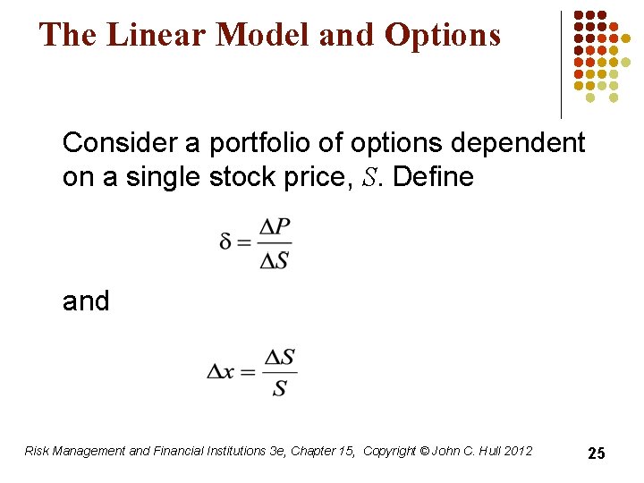
The Linear Model and Options Consider a portfolio of options dependent on a single stock price, S. Define and Risk Management and Financial Institutions 3 e, Chapter 15, Copyright © John C. Hull 2012 25

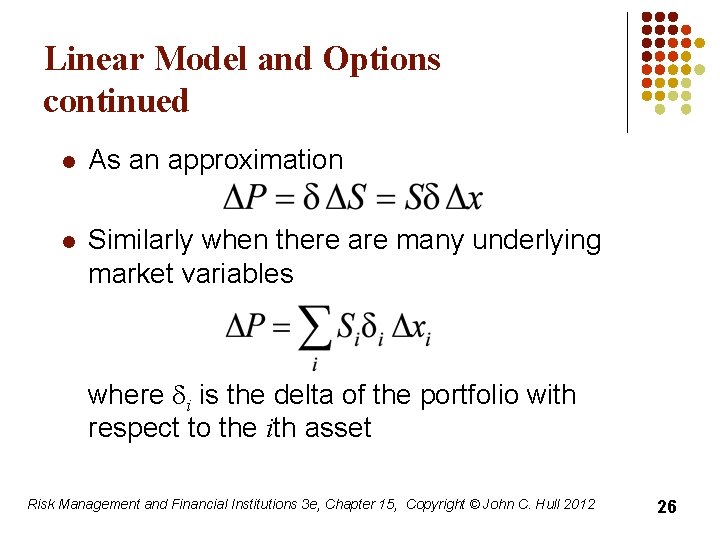
Linear Model and Options continued l As an approximation l Similarly when there are many underlying market variables where di is the delta of the portfolio with respect to the ith asset Risk Management and Financial Institutions 3 e, Chapter 15, Copyright © John C. Hull 2012 26

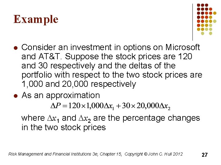
Example l l Consider an investment in options on Microsoft and AT&T. Suppose the stock prices are 120 and 30 respectively and the deltas of the portfolio with respect to the two stock prices are 1, 000 and 20, 000 respectively As an approximation where Dx 1 and Dx 2 are the percentage changes in the two stock prices Risk Management and Financial Institutions 3 e, Chapter 15, Copyright © John C. Hull 2012 27

But the Distribution of the Daily Return on an Option is not Normal The linear model fails to capture skewness in the probability distribution of the portfolio value. Risk Management and Financial Institutions 3 e, Chapter 15, Copyright © John C. Hull 2012 28

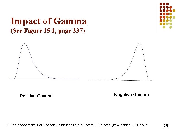
Impact of Gamma (See Figure 15. 1, page 337) Positive Gamma Negative Gamma Risk

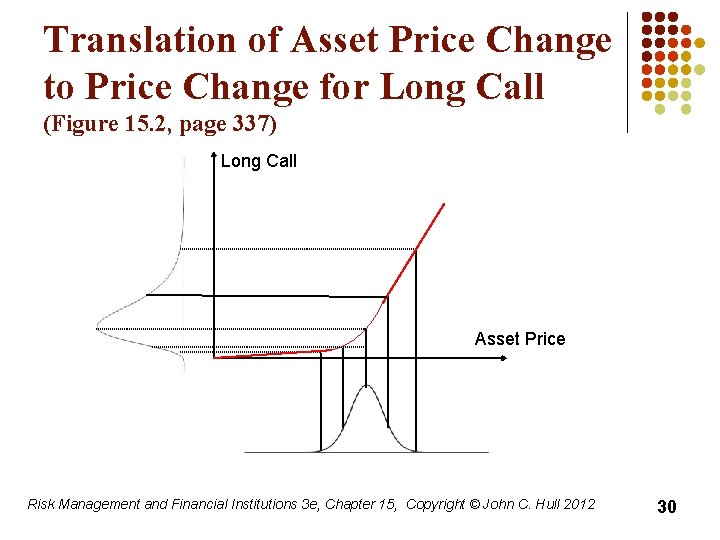
Translation of Asset Price Change to Price Change for Long Call (Figure 15. 2, page 337) Long Call Asset Price Risk Management and Financial Institutions 3 e, Chapter 15, Copyright © John C. Hull 2012 30

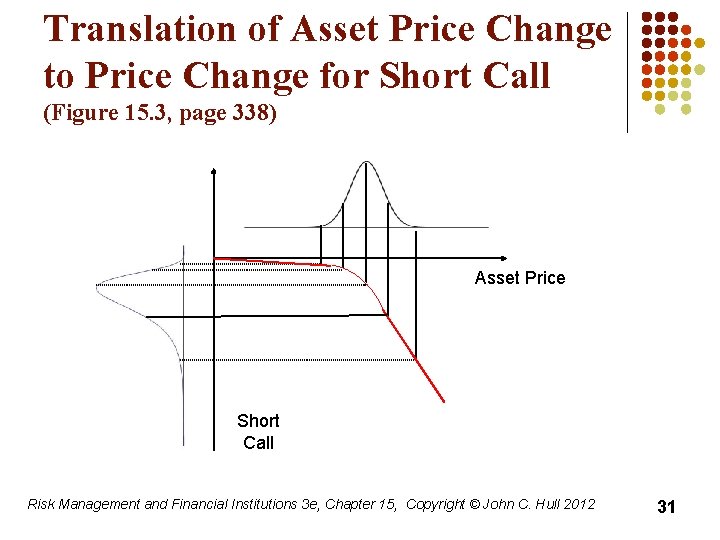
Translation of Asset Price Change to Price Change for Short Call (Figure 15. 3, page 338) Asset Price Short Call Risk Management and Financial Institutions 3 e, Chapter 15, Copyright © John C. Hull 2012 31

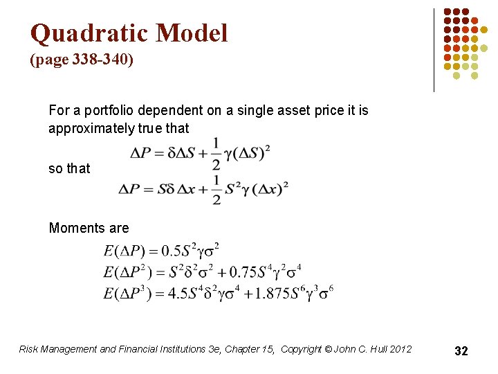
Quadratic Model (page 338 -340) For a portfolio dependent on a single asset price it is approximately true that so that Moments are Risk Management and Financial Institutions 3 e, Chapter 15, Copyright © John C. Hull 2012 32

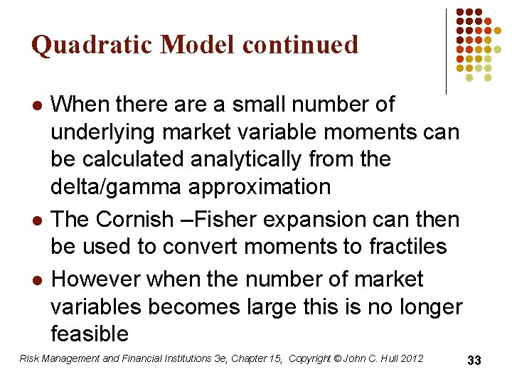
Quadratic Model continued l l l When there a small number of underlying market variable moments can be calculated analytically from the delta/gamma approximation The Cornish –Fisher expansion can then be used to convert moments to fractiles However when the number of market variables becomes large this is no longer feasible Risk Management and Financial Institutions 3 e, Chapter 15, Copyright © John C. Hull 2012 33

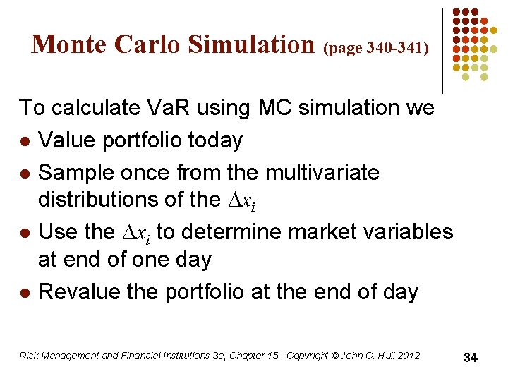
Monte Carlo Simulation (page 340 -341) To calculate Va. R using MC simulation we l Value portfolio today l Sample once from the multivariate distributions of the Dxi l Use the Dxi to determine market variables at end of one day l Revalue the portfolio at the end of day Risk Management and Financial Institutions 3 e, Chapter 15, Copyright © John C. Hull 2012 34

Monte Carlo Simulation continued l l Calculate DP Repeat many times to build up a probability distribution for DP Va. R is the appropriate fractile of the distribution times square root of N For example, with 1, 000 trial the 1 percentile is the 10 th worst case. Risk Management and Financial Institutions 3 e, Chapter 15, Copyright © John C. Hull 2012 35

Speeding up Calculations with the Partial Simulation Approach l l Use the approximate delta/gamma relationship between DP and the Dxi to calculate the change in value of the portfolio This is also a way of speeding up computations in the historical simulation approach Risk Management and Financial Institutions 3 e, Chapter 15, Copyright © John C. Hull 2012 36

Alternative to Normal Distribution Assumption in Monte Carlo l l In a Monte Carlo simulation we can assume non-normal distributions for the xi (e. g. , a multivariate t-distribution) Can also use a Gaussian or other copula model in conjunction with empirical distributions Risk Management and Financial Institutions 3 e, Chapter 15, Copyright © John C. Hull 2012 37

Model Building vs Historical Simulation Model building approach can be used for investment portfolios where there are no derivatives, but it does not usually work when for portfolios where l l There are derivatives Positions are close to delta neutral Risk Management and Financial Institutions 3 e, Chapter 15, Copyright © John C. Hull 2012 38