Market Risk Va R Historical Simulation Approach N

Market Risk Va. R: Historical Simulation Approach N. Gershun

Historical Simulation • Collect data on the daily movements in all market variables. • The first simulation trial assumes that the percentage changes in all market variables are as on the first day • The second simulation trial assumes that the percentage changes in all market variables are as on the second day • and so on

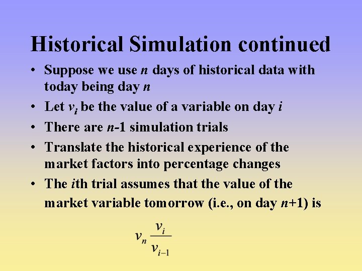
Historical Simulation continued • Suppose we use n days of historical data with today being day n • Let vi be the value of a variable on day i • There are n-1 simulation trials • Translate the historical experience of the market factors into percentage changes • The ith trial assumes that the value of the market variable tomorrow (i. e. , on day n+1) is

Historical Simulation continued • Rank the n-1 resulting values • Va. R is the required percentile rank

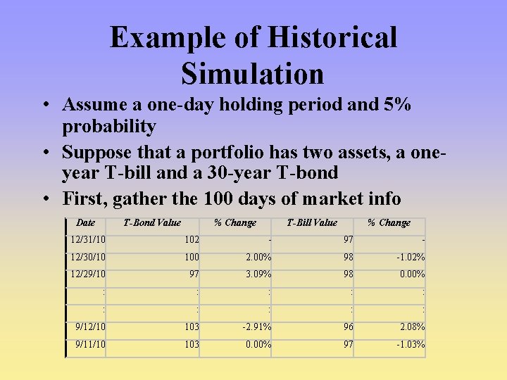
Example of Historical Simulation • Assume a one-day holding period and 5% probability • Suppose that a portfolio has two assets, a oneyear T-bill and a 30 -year T-bond • First, gather the 100 days of market info Date T-Bond Value % Change T-Bill Value % Change 12/31/10 102 - 97 - 12/30/10 100 2. 00% 98 -1. 02% 12/29/10 97 3. 09% 98 0. 00% : : : 9/12/10 103 -2. 91% 96 2. 08% 9/11/10 103 0. 00% 97 -1. 03%

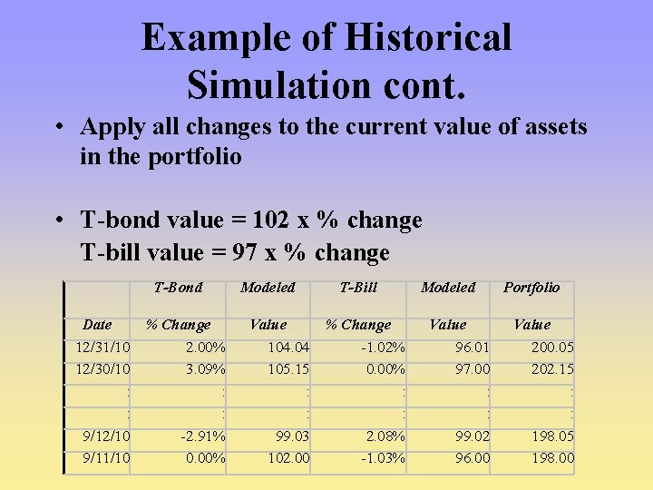
Example of Historical Simulation cont. • Apply all changes to the current value of assets in the portfolio • T-bond value = 102 x % change T-bill value = 97 x % change T-Bond Date % Change 12/31/10 2. 00% 12/30/10 3. 09% : : 9/12/10 -2. 91% 9/11/10 0. 00% Modeled T-Bill Value % Change 104. 04 -1. 02% 105. 15 0. 00% : : 99. 03 2. 08% 102. 00 -1. 03% Modeled Value 96. 01 97. 00 : : 99. 02 96. 00 Portfolio Value 200. 05 202. 15 : : 198. 05 198. 00

Example of Historical Simulation cont. • Rank the resulting 100 portfolio values • The 5 th lowest portfolio value is the Va. R Rank 1 2 3 4 Date 11/12/10 12/1/10 10/17/10 10/13/10 Value 195. 45 196. 24 197. 13 197. 60 5 9/11/10 198. 00 : : 99 100 : : 12/8/10 9/25/10 : : 202. 15 203. 00

Notes on Historical Simulation • Historical simulation is relatively easy to do: Only requires knowing the market factors and having the historical information • Correlations between the market factors are implicit in this method because we are using historical information • In our example, short bonds and long bonds would typically move in the same direction

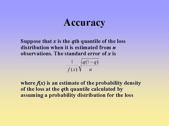
Accuracy Suppose that x is the qth quantile of the loss distribution when it is estimated from n observations. The standard error of x is where f(x) is an estimate of the probability density of the loss at the qth quantile calculated by assuming a probability distribution for the loss

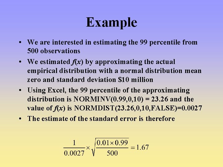
Example • We are interested in estimating the 99 percentile from 500 observations • We estimated f(x) by approximating the actual empirical distribution with a normal distribution mean zero and standard deviation $10 million • Using Excel, the 99 percentile of the approximating distribution is NORMINV(0. 99, 0, 10) = 23. 26 and the value of f(x) is NORMDIST(23. 26, 0, 10, FALSE)=0. 0027 • The estimate of the standard error is therefore

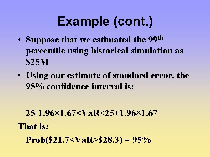
Example (cont. ) • Suppose that we estimated the 99 th percentile using historical simulation as $25 M • Using our estimate of standard error, the 95% confidence interval is: 25 -1. 96× 1. 67<Va. R<25+1. 96× 1. 67 That is: Prob($21. 7<Va. R>$28. 3) = 95%

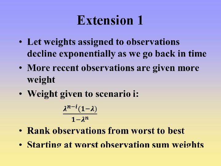
Extension 1 •

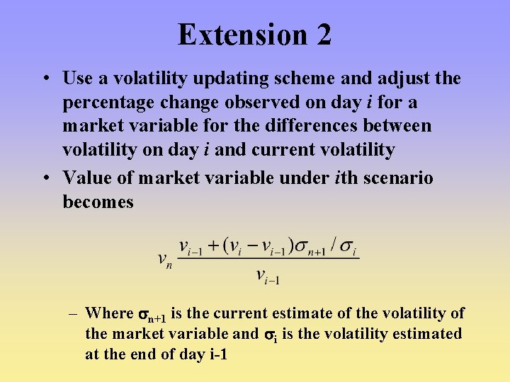
Extension 2 • Use a volatility updating scheme and adjust the percentage change observed on day i for a market variable for the differences between volatility on day i and current volatility • Value of market variable under ith scenario becomes – Where n+1 is the current estimate of the volatility of the market variable and i is the volatility estimated at the end of day i-1

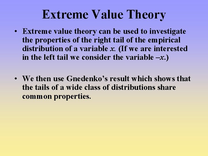
Extreme Value Theory • Extreme value theory can be used to investigate the properties of the right tail of the empirical distribution of a variable x. (If we are interested in the left tail we consider the variable –x. ) • We then use Gnedenko’s result which shows that the tails of a wide class of distributions share common properties.

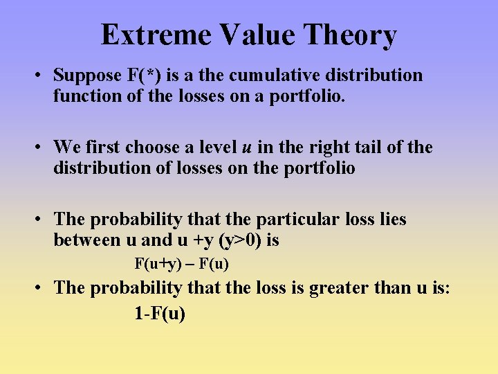
Extreme Value Theory • Suppose F(*) is a the cumulative distribution function of the losses on a portfolio. • We first choose a level u in the right tail of the distribution of losses on the portfolio • The probability that the particular loss lies between u and u +y (y>0) is F(u+y) – F(u) • The probability that the loss is greater than u is: 1 -F(u)

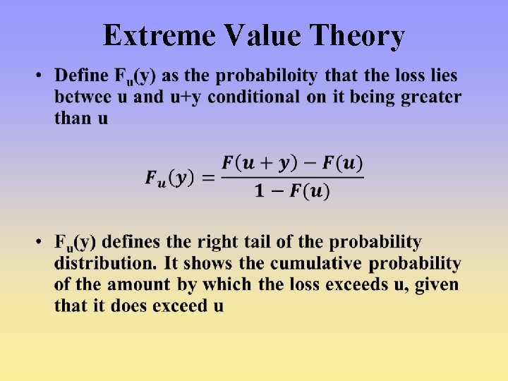
Extreme Value Theory •

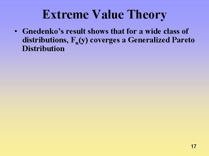
Extreme Value Theory • Gnedenko’s result shows that for a wide class of distributions, Fu(y) coverges a Generalized Pareto Distribution 17

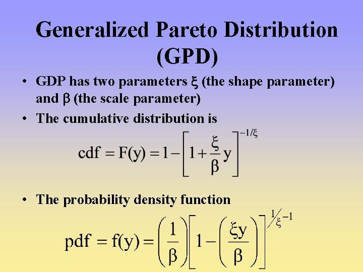
Generalized Pareto Distribution (GPD) • GDP has two parameters (the shape parameter) and (the scale parameter) • The cumulative distribution is • The probability density function

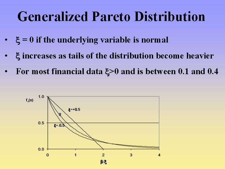
Generalized Pareto Distribution • = 0 if the underlying variable is normal • increases as tails of the distribution become heavier • For most financial data >0 and is between 0. 1 and 0. 4 fx(x) =+0. 5 0 =-0. 5 /

Generalized Pareto Distribution (cont). • G. P. D. is appropriate distribution for independent observations of excesses over defined thresholds • GPD can be used to predict extreme portfolio losses

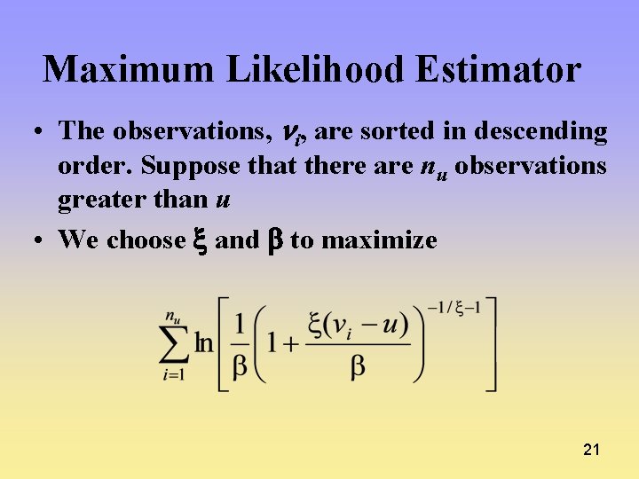
Maximum Likelihood Estimator • The observations, i, are sorted in descending order. Suppose that there are nu observations greater than u • We choose and to maximize 21

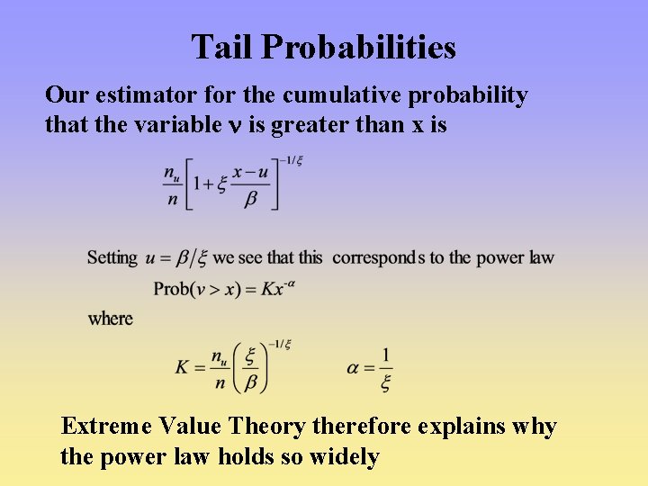
Tail Probabilities Our estimator for the cumulative probability that the variable is greater than x is Extreme Value Theory therefore explains why the power law holds so widely

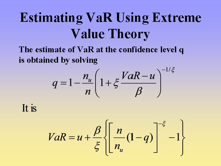
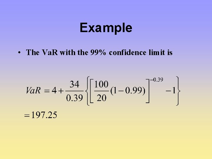
Estimating Va. R Using Extreme Value Theory The estimate of Va. R at the confidence level q is obtained by solving

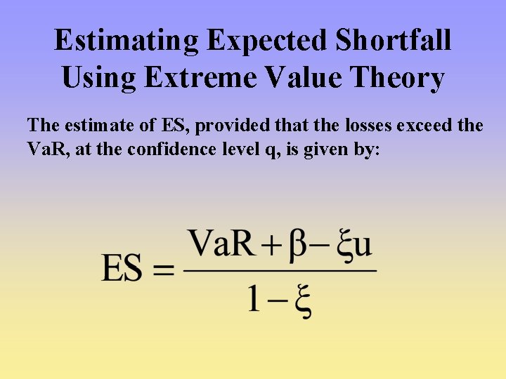
Estimating Expected Shortfall Using Extreme Value Theory The estimate of ES, provided that the losses exceed the Va. R, at the confidence level q, is given by:

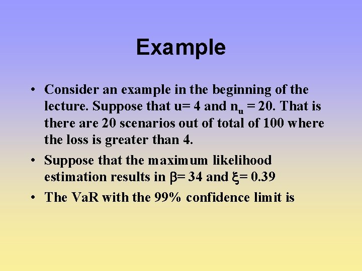
Example • Consider an example in the beginning of the lecture. Suppose that u= 4 and nu = 20. That is there are 20 scenarios out of total of 100 where the loss is greater than 4. • Suppose that the maximum likelihood estimation results in = 34 and = 0. 39 • The Va. R with the 99% confidence limit is

Example • The Va. R with the 99% confidence limit is