MARKET RISK MANAGEMENT MEASUREMENT MONTE CARLO SIMULATION Real

MARKET RISK MANAGEMENT: MEASUREMENT: MONTE CARLO SIMULATION Real Data Monte Carlo Simulation BAHATTIN BUYUKSAHIN AND CELSO BRUNETTI 1

REAL DATA Returns Distribution Stylized Facts

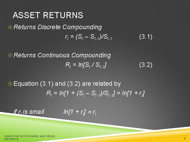
ASSET RETURNS Returns Discrete Compounding rt = (St – St-1)/St-1 (3. 1) Returns Continuous Compounding Rt = ln[St / St-1] (3. 2) Equation (3. 1) and (3. 2) are related by Rt = ln[1 + (St – St-1)/St-1] = ln[1 + rt] if rt is small BAHATTIN BUYUKSAHIN AND CELSO BRUNETTI ln[1 + rt] rt 3

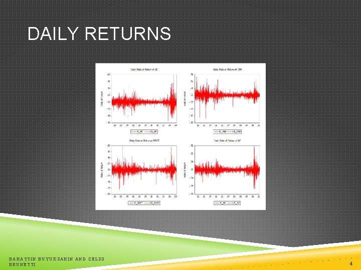
DAILY RETURNS BAHATTIN BUYUKSAHIN AND CELSO BRUNETTI 4

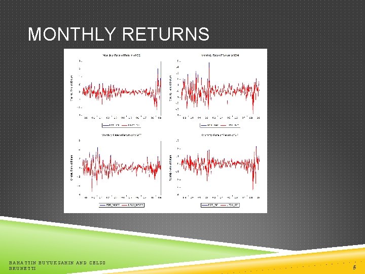
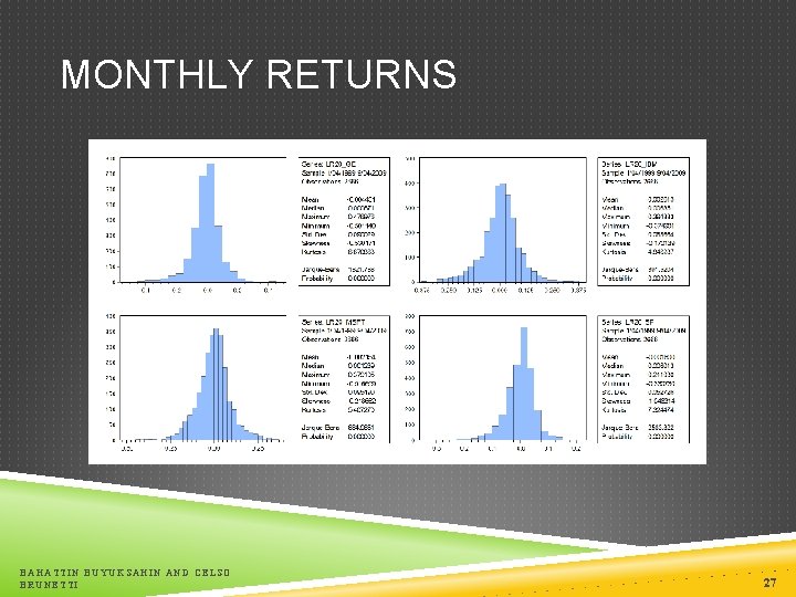
MONTHLY RETURNS BAHATTIN BUYUKSAHIN AND CELSO BRUNETTI 5

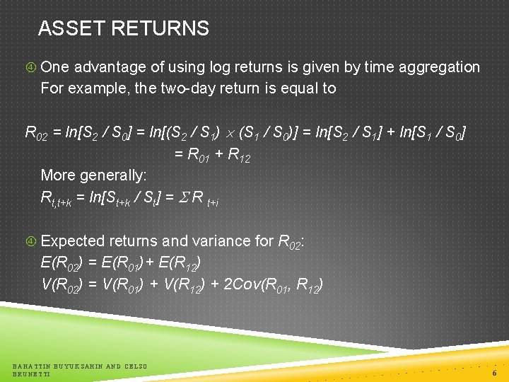
ASSET RETURNS One advantage of using log returns is given by time aggregation For example, the two-day return is equal to R 02 = ln[S 2 / S 0] = ln[(S 2 / S 1) (S 1 / S 0)] = ln[S 2 / S 1] + ln[S 1 / S 0] = R 01 + R 12 More generally: Rt, t+k = ln[St+k / St] = R t+i Expected returns and variance for R 02: E(R 02) = E(R 01)+ E(R 12) V(R 02) = V(R 01) + V(R 12) + 2 Cov(R 01, R 12) BAHATTIN BUYUKSAHIN AND CELSO BRUNETTI 6

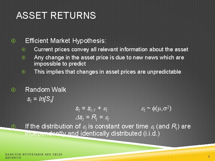
ASSET RETURNS Efficient Market Hypothesis: Current prices convey all relevant information about the asset Any change in the asset price is due to news which are impossible to predict This implies that changes in asset prices are unpredictable Random Walk st = ln[St] st = st-1 + t t ~ ( , 2) st = Rt = t If the distribution of t is constant over time t (and Rt) are independently and identically distributed (i. i. d. ) BAHATTIN BUYUKSAHIN AND CELSO BRUNETTI 7

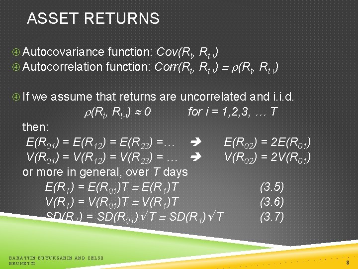
ASSET RETURNS Autocovariance function: Cov(Rt, Rt-i) Autocorrelation function: Corr(Rt, Rt-i) If we assume that returns are uncorrelated and i. i. d. (Rt, Rt-i) 0 for i = 1, 2, 3, … T then: E(R 01) = E(R 12) = E(R 23) =… E(R 02) = 2 E(R 01) V(R 01) = V(R 12) = V(R 23) = … V(R 02) = 2 V(R 01) or more in general, over T days E(RT) = E(R 01)T E(R 1)T (3. 5) V(RT) = V(R 01)T V(R 1)T (3. 6) SD(RT) = SD(R 01) T SD(R 1) T (3. 7) BAHATTIN BUYUKSAHIN AND CELSO BRUNETTI 8

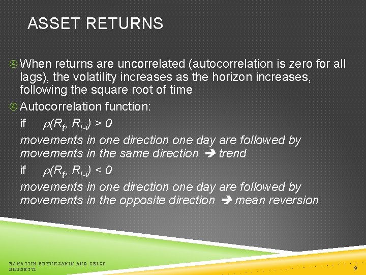
ASSET RETURNS When returns are uncorrelated (autocorrelation is zero for all lags), the volatility increases as the horizon increases, following the square root of time Autocorrelation function: if (Rt, Rt-i) > 0 movements in one direction one day are followed by movements in the same direction trend if (Rt, Rt-i) < 0 movements in one direction one day are followed by movements in the opposite direction mean reversion BAHATTIN BUYUKSAHIN AND CELSO BRUNETTI 9

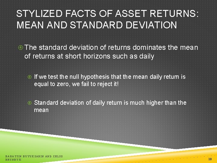
STYLIZED FACTS OF ASSET RETURNS: MEAN AND STANDARD DEVIATION The standard deviation of returns dominates the mean of returns at short horizons such as daily If we test the null hypothesis that the mean daily return is equal to zero, we fail to reject it! Standard deviation of daily return is much higher than the mean BAHATTIN BUYUKSAHIN AND CELSO BRUNETTI 10

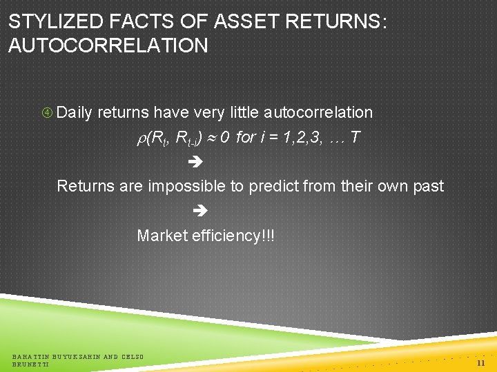
STYLIZED FACTS OF ASSET RETURNS: AUTOCORRELATION Daily returns have very little autocorrelation (Rt, Rt-i) 0 for i = 1, 2, 3, … T Returns are impossible to predict from their own past Market efficiency!!! BAHATTIN BUYUKSAHIN AND CELSO BRUNETTI 11

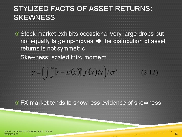
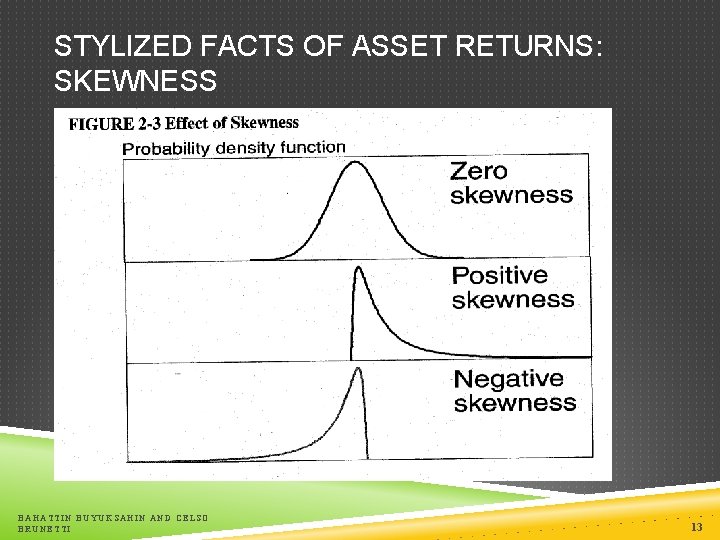
STYLIZED FACTS OF ASSET RETURNS: SKEWNESS Stock market exhibits occasional very large drops but not equally large up-moves the distribution of asset returns is not symmetric Skewness: scaled third moment FX market tends to show less evidence of skewness BAHATTIN BUYUKSAHIN AND CELSO BRUNETTI 12

STYLIZED FACTS OF ASSET RETURNS: SKEWNESS BAHATTIN BUYUKSAHIN AND CELSO BRUNETTI 13

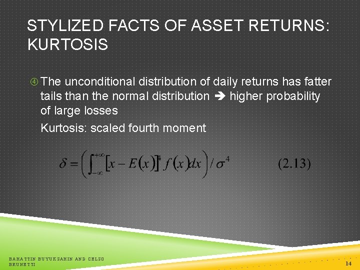
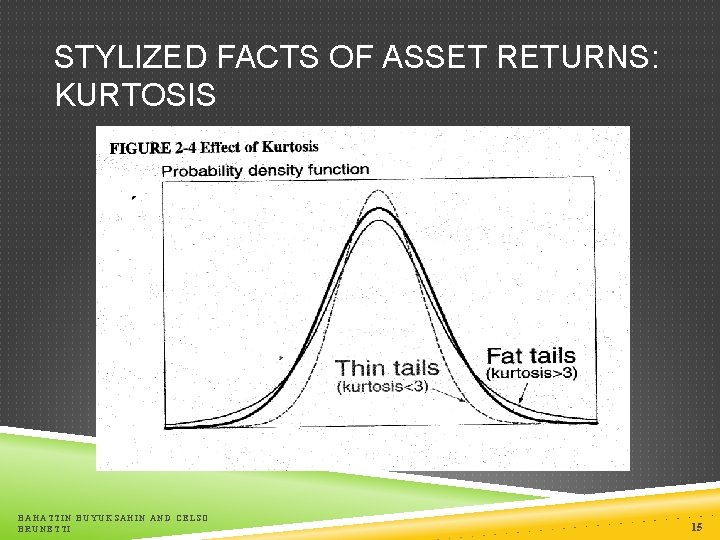
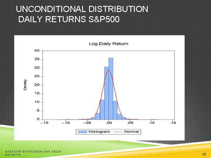
STYLIZED FACTS OF ASSET RETURNS: KURTOSIS The unconditional distribution of daily returns has fatter tails than the normal distribution higher probability of large losses Kurtosis: scaled fourth moment BAHATTIN BUYUKSAHIN AND CELSO BRUNETTI 14

STYLIZED FACTS OF ASSET RETURNS: KURTOSIS BAHATTIN BUYUKSAHIN AND CELSO BRUNETTI 15

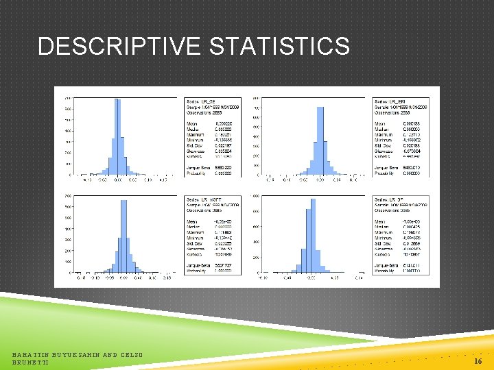
DESCRIPTIVE STATISTICS BAHATTIN BUYUKSAHIN AND CELSO BRUNETTI 16

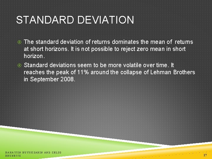
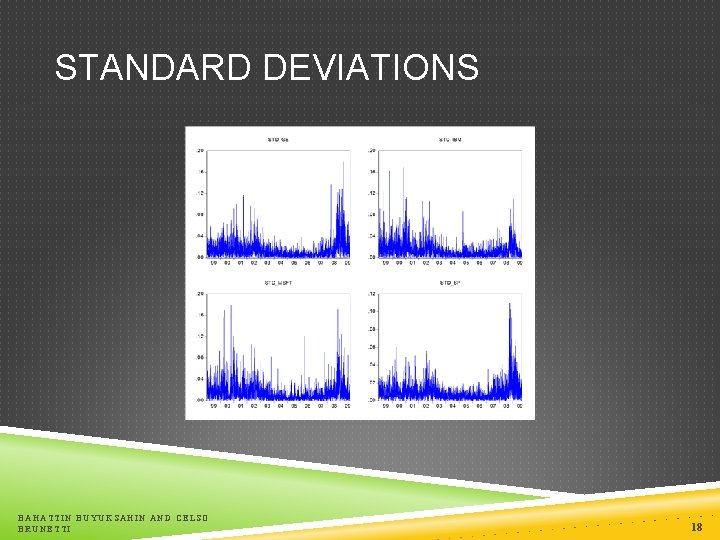
STANDARD DEVIATION The standard deviation of returns dominates the mean of returns at short horizons. It is not possible to reject zero mean in short horizon. Standard deviations seem to be more volatile over time. It reaches the peak of 11% around the collapse of Lehman Brothers in September 2008. BAHATTIN BUYUKSAHIN AND CELSO BRUNETTI 17

STANDARD DEVIATIONS BAHATTIN BUYUKSAHIN AND CELSO BRUNETTI 18

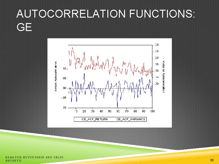
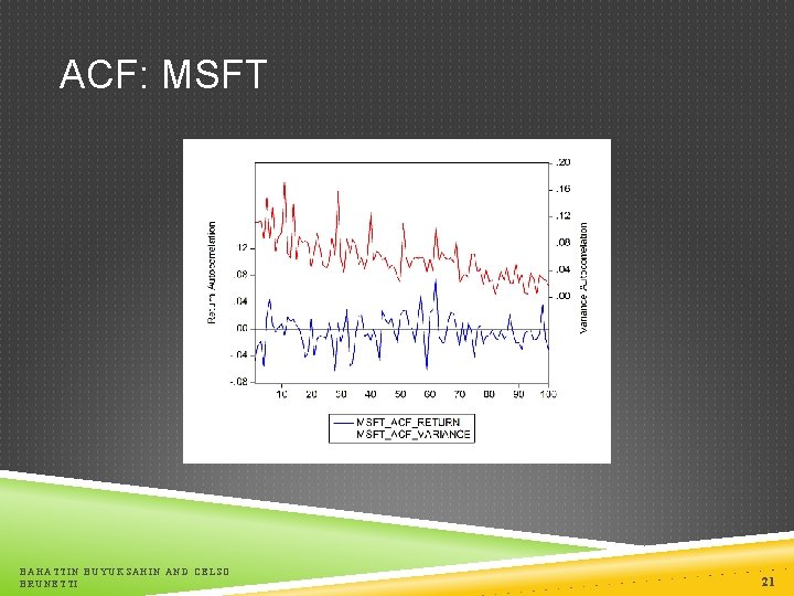
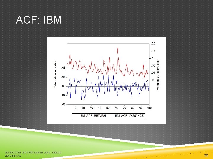
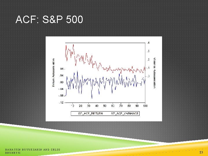
STYLIZED FACTS OF ASSET RETURNS: SQUARED RETURNS Squared returns variance 2 = E(x 2) – [E(x)]2 st = Rt = t t ~ (0, 2) E(Rt) = 0 2 = E(x 2) Squared returns exhibit positive autocorrelation (R 2 t, R 2 t-i) > 0 for i = 1, 2, 3, … T The autocorrelations of squared returns tend to be positive for short lags and decay exponentially to zero as the number of lags increases. BAHATTIN BUYUKSAHIN AND CELSO BRUNETTI 19

AUTOCORRELATION FUNCTIONS: GE BAHATTIN BUYUKSAHIN AND CELSO BRUNETTI 20

ACF: MSFT BAHATTIN BUYUKSAHIN AND CELSO BRUNETTI 21

ACF: IBM BAHATTIN BUYUKSAHIN AND CELSO BRUNETTI 22

ACF: S&P 500 BAHATTIN BUYUKSAHIN AND CELSO BRUNETTI 23

STYLIZED FACTS OF ASSET RETURNS: LEVERAGE EFFECT Equity and equity indices display negative correlation between variance and returns Leverage effect A drop in the stock price will increase the leverage of the firm and therefore the risk (variance) BAHATTIN BUYUKSAHIN AND CELSO BRUNETTI 24

STYLIZED FACTS OF ASSET RETURNS: CORRELATION BETWEEN ASSETS Correlation between assets is not constant over time – i. e. it changes Empirical evidence shows that assets are more correlated during crashes!!! Covariance: E(xy) = E[(x – E(x)) (y – E(y))] if E(x) = 0 and E(y) = 0 E(xy) = E(x y) Cov(Ri, t, Rj, t) = E(Ri, t, Rj, t) Covariance between asset returns may be estimated by the product of the returns BAHATTIN BUYUKSAHIN AND CELSO BRUNETTI 25

STYLIZED FACTS OF ASSET RETURNS: RETURN HORIZON As the return horizon increases, the unconditional return distribution changes and looks increasingly like a normal distribution BAHATTIN BUYUKSAHIN AND CELSO BRUNETTI 26

MONTHLY RETURNS BAHATTIN BUYUKSAHIN AND CELSO BRUNETTI 27

UNCONDITIONAL DISTRIBUTION DAILY RETURNS S&P 500 BAHATTIN BUYUKSAHIN AND CELSO BRUNETTI 28

MONTE CARLO & SIMULATION

RANDOM VARIABLES

MONTE CARLO SIMULATION Monte Carlo simulation involve creating artificial random variables, whose time path is not predictable. Any variable whose value changes over time in an unpredictable way is said to follow a stochastic process A Markov process is a particular type of stochastic process where only the present value of a variable is relevant for predicting the future. BAHATTIN BUYUKSAHIN AND CELSO BRUNETTI 31

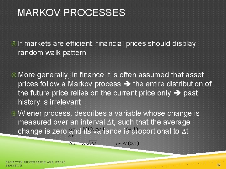
MARKOV PROCESSES If markets are efficient, financial prices should display random walk pattern More generally, in finance it is often assumed that asset prices follow a Markov process the entire distribution of the future price relies on the current price only past history is irrelevant Wiener process: describes a variable whose change is measured over an interval t, such that the average change is zero and its variance is proportional to t BAHATTIN BUYUKSAHIN AND CELSO BRUNETTI 32

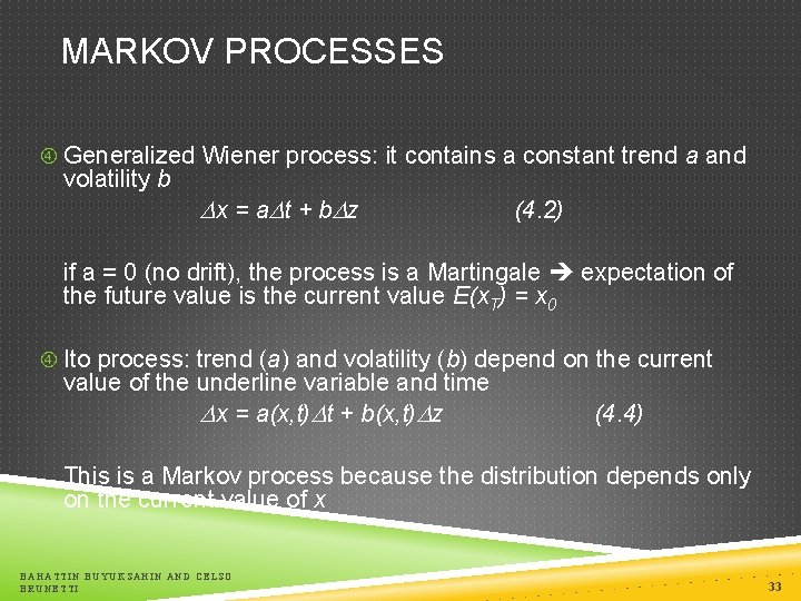
MARKOV PROCESSES Generalized Wiener process: it contains a constant trend a and volatility b x = a t + b z (4. 2) if a = 0 (no drift), the process is a Martingale expectation of the future value is the current value E(x. T) = x 0 Ito process: trend (a) and volatility (b) depend on the current value of the underline variable and time x = a(x, t) t + b(x, t) z (4. 4) This is a Markov process because the distribution depends only on the current value of x BAHATTIN BUYUKSAHIN AND CELSO BRUNETTI 33

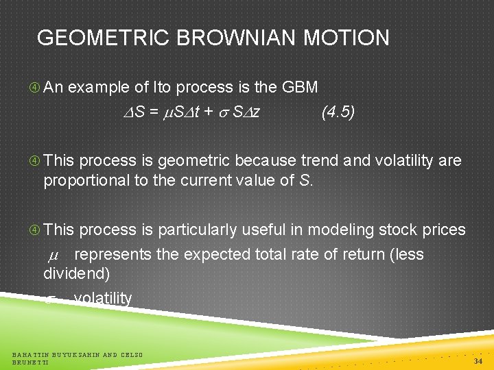
GEOMETRIC BROWNIAN MOTION An example of Ito process is the GBM S = S t + S z (4. 5) This process is geometric because trend and volatility are proportional to the current value of S. This process is particularly useful in modeling stock prices represents the expected total rate of return (less dividend) volatility BAHATTIN BUYUKSAHIN AND CELSO BRUNETTI 34

BAHATTIN BUYUKSAHIN AND CELSO BRUNETTI 35

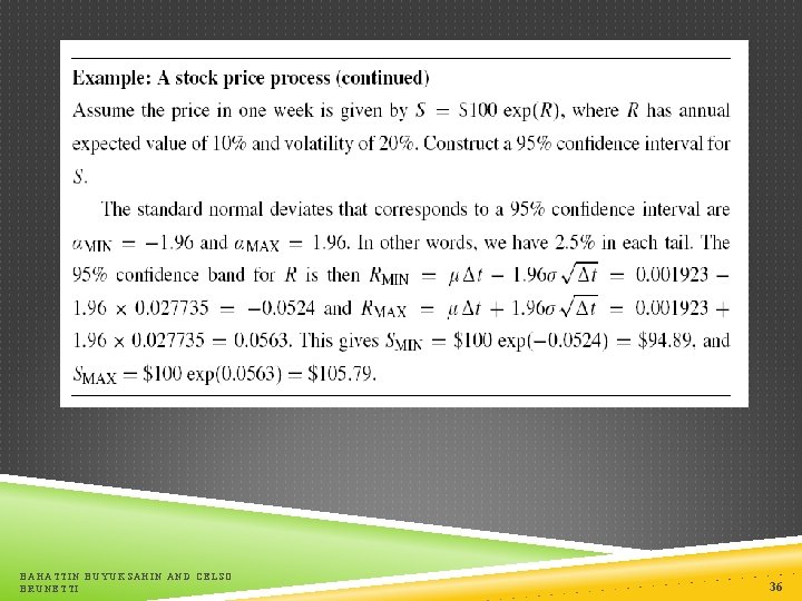
BAHATTIN BUYUKSAHIN AND CELSO BRUNETTI 36

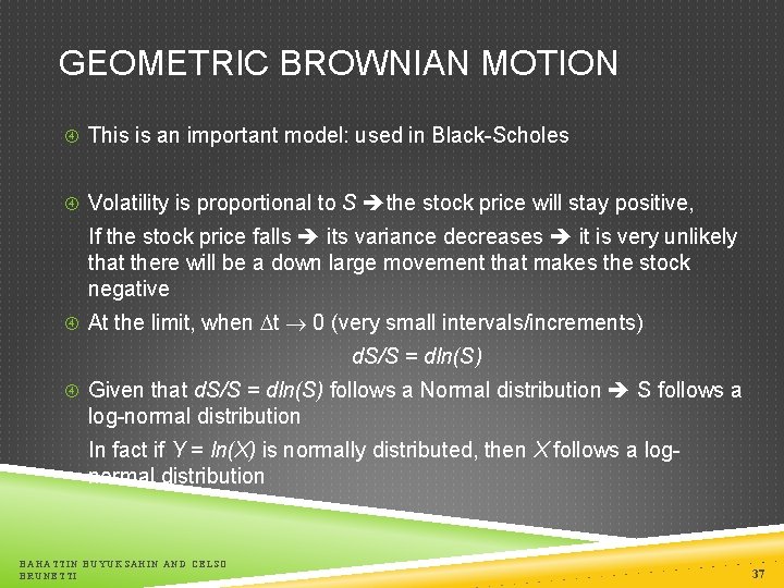
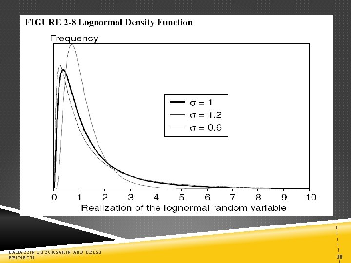
GEOMETRIC BROWNIAN MOTION This is an important model: used in Black-Scholes Volatility is proportional to S the stock price will stay positive, If the stock price falls its variance decreases it is very unlikely that there will be a down large movement that makes the stock negative At the limit, when t 0 (very small intervals/increments) d. S/S = dln(S) Given that d. S/S = dln(S) follows a Normal distribution S follows a log-normal distribution In fact if Y = ln(X) is normally distributed, then X follows a lognormal distribution BAHATTIN BUYUKSAHIN AND CELSO BRUNETTI 37

BAHATTIN BUYUKSAHIN AND CELSO BRUNETTI 38

GEOMETRIC BROWNIAN MOTION The GBM implies that over an interval of time, T – t = the ln of the final price is given by Should we choose a Normal distribution or a log- Normal for our price process? It depends on the time horizon Short time periods (such as a day) it does not matter which of the two distributions we choose Long horizons (such as years) it is better to adopt the log- normal prices will not be negative BAHATTIN BUYUKSAHIN AND CELSO BRUNETTI 39

SIMULATION BAHATTIN BUYUKSAHIN AND CELSO BRUNETTI 40

BAHATTIN BUYUKSAHIN AND CELSO BRUNETTI 41

BAHATTIN BUYUKSAHIN AND CELSO BRUNETTI 42

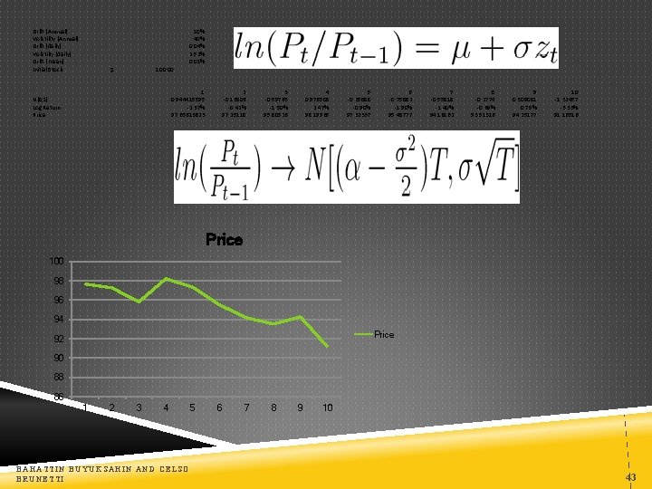
Drift (Annual) Volatility (Annual) Drift (daily) Volatilty (daily) Drift (mean) Initial Stock $ 100. 00 10% 40% 0. 04% 2. 52% 0. 01% 1 -0. 944415595 -2. 37% 97. 65613823 N(0, 1) Log Return Price 2 -0. 16806 -0. 42% 97. 25118 3 -0. 59763 -1. 50% 95. 80526 4 0. 976508 2. 47% 98. 19965 5 -0. 35888 -0. 90% 97. 32337 6 -0. 75882 -1. 90% 95. 48777 7 -0. 55818 -1. 40% 94. 16162 8 -0. 2774 -0. 69% 93. 51316 9 0. 309081 0. 79% 94. 25177 10 -1. 32457 -3. 33% 91. 16516 Price 100 98 96 94 Price 92 90 88 86 1 2 3 4 BAHATTIN BUYUKSAHIN AND CELSO BRUNETTI 5 6 7 8 9 10 43

SIMULATION Remember: We can replicate a Monte Carlo experiment many times. Each time we will generate a new path Initial values may affect the results Seed: it allows to generate the same random numbers BAHATTIN BUYUKSAHIN AND CELSO BRUNETTI 44

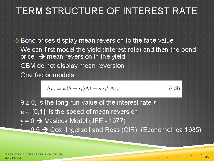
TERM STRUCTURE OF INTEREST RATE Bond prices display mean reversion to the face value We can first model the yield (interest rate) and then the bond price mean reversion in the yield GBM do not display mean reversion One factor models 0, is the long-run value of the interest rate r [0, 1], is the speed of mean reversion = 0 Vasicek Model (JFE - 1977) = 0. 5 Cox, Ingersoll and Ross (CIR), (Econometrica 1985) BAHATTIN BUYUKSAHIN AND CELSO BRUNETTI 45

TERM STRUCTURE OF INTEREST RATE In C-I-R’s model the stochastic term is proportional to r½ indicating that, as the short term interest rate increases, its standard deviation increases In C-I-R’s model interest rates are always positive. A negative value is implausible for nominal interest rates but not for real rates In Vasicek the short term interest rate can be negative: implausible for nominal but not for real rates Vasicek and C-I-R both accommodate rising, falling and single humped structure In both Vasicek and C-I-R the short term interest rate converges towards a long term interest rate which is constant and independent from r However, in practice, long rate is quite variable two-factor models BAHATTIN BUYUKSAHIN AND CELSO BRUNETTI 46

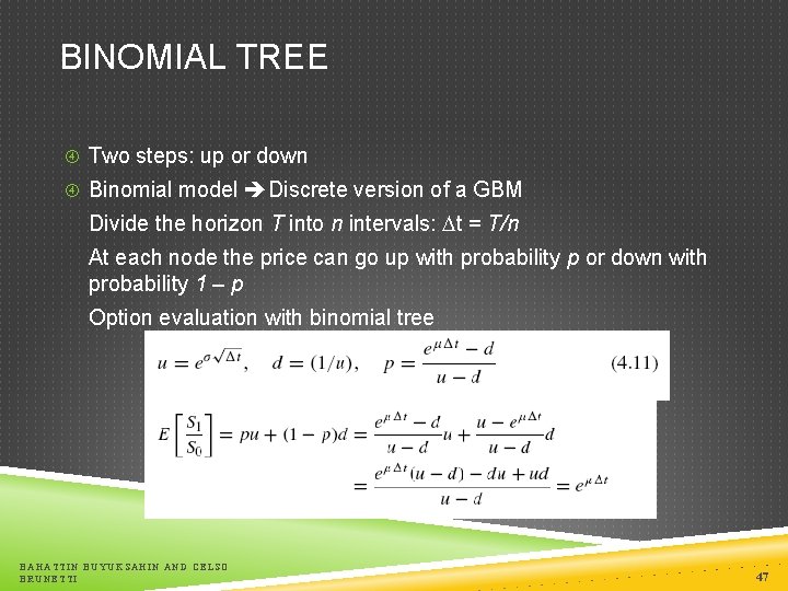
BINOMIAL TREE Two steps: up or down Binomial model Discrete version of a GBM Divide the horizon T into n intervals: t = T/n At each node the price can go up with probability p or down with probability 1 – p Option evaluation with binomial tree BAHATTIN BUYUKSAHIN AND CELSO BRUNETTI 47

BINOMIAL TREE BAHATTIN BUYUKSAHIN AND CELSO BRUNETTI 48

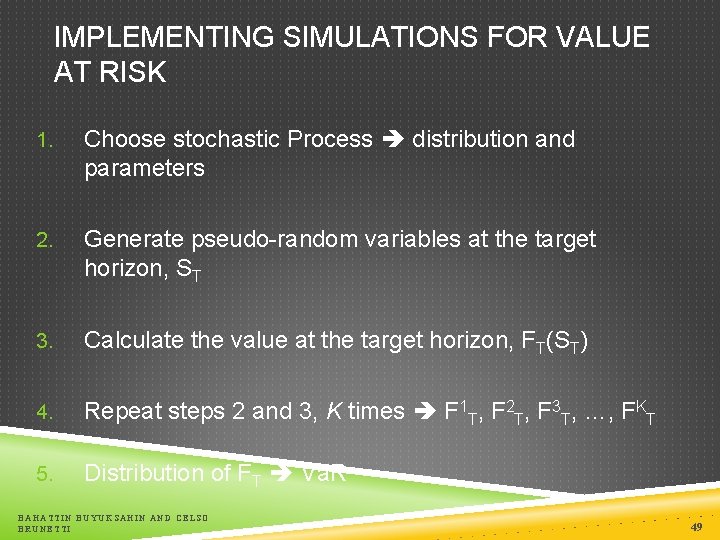
IMPLEMENTING SIMULATIONS FOR VALUE AT RISK 1. Choose stochastic Process distribution and parameters 2. Generate pseudo-random variables at the target horizon, ST 3. Calculate the value at the target horizon, FT(ST) 4. Repeat steps 2 and 3, K times F 1 T, F 2 T, F 3 T, …, FKT 5. Distribution of FT Va. R BAHATTIN BUYUKSAHIN AND CELSO BRUNETTI 49

IMPLEMENTING SIMULATIONS Simulations for option pricing: Risk-neutral approach the price grows at the risk-free rate model based simulation Simulations for Va. R: physical distribution – i. e. the actual distribution Sampling variability: even with K large, the empirical distribution of ST will only be an approximation of the true distribution Monte Carlo: Independent draws standard error is inversely related to K BAHATTIN BUYUKSAHIN AND CELSO BRUNETTI 50

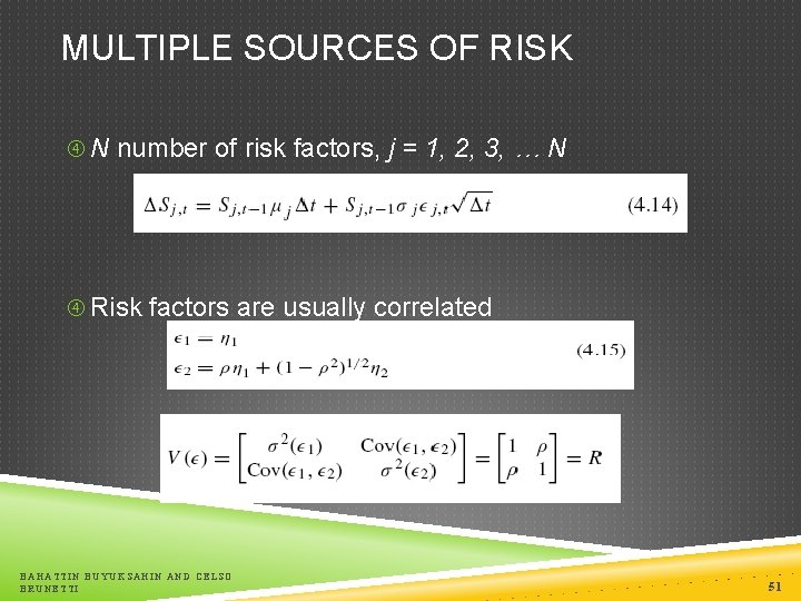
MULTIPLE SOURCES OF RISK N number of risk factors, j = 1, 2, 3, … N Risk factors are usually correlated BAHATTIN BUYUKSAHIN AND CELSO BRUNETTI 51

MULTIPLE SOURCES OF RISK If we have N risk factors, we have N(N – 1)/2 covariances A portfolio with 100 assets will have to consider 4, 950 covariances! We only consider the main risk factors BAHATTIN BUYUKSAHIN AND CELSO BRUNETTI 52