Marginal Structural Models Robins Hernan Brumback 2000 Hernan

Marginal Structural Models Robins, Hernan, Brumback (2000) Hernan, Brumback, Robins (2000)

MSM and Causal Inference in Epidemiology • First sections describe the problem of timedependent confounding. • Later sections describe MSM. • Outcome of interest is a binary Y at the end of follow-up. • Treatment may change over time. • There are time-dependent confounders.

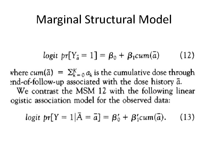
Marginal Structural Model

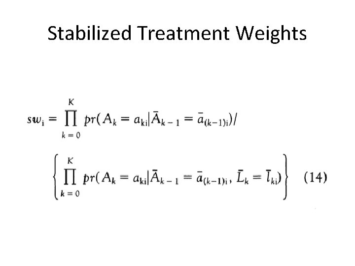
Stabilized Treatment Weights

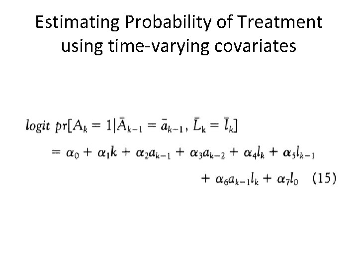
Estimating Probability of Treatment using time-varying covariates

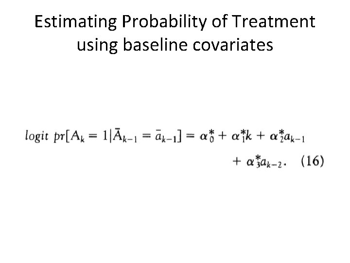
Estimating Probability of Treatment using baseline covariates

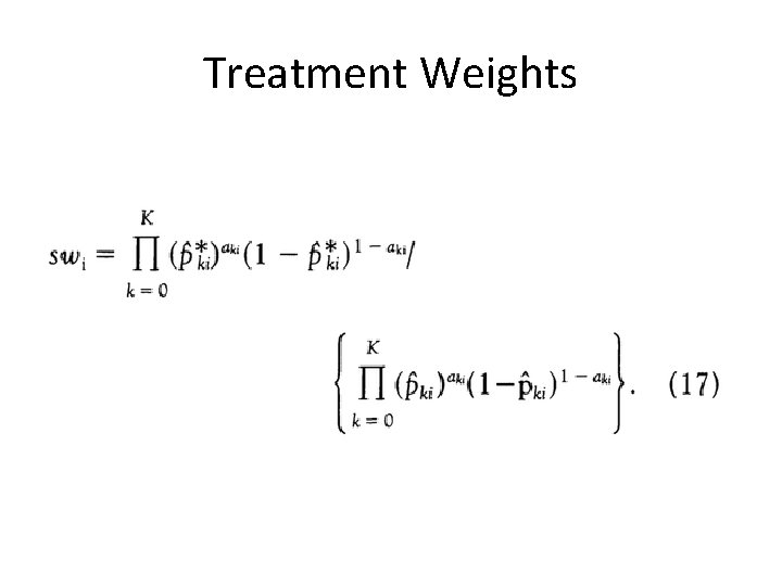
Treatment Weights

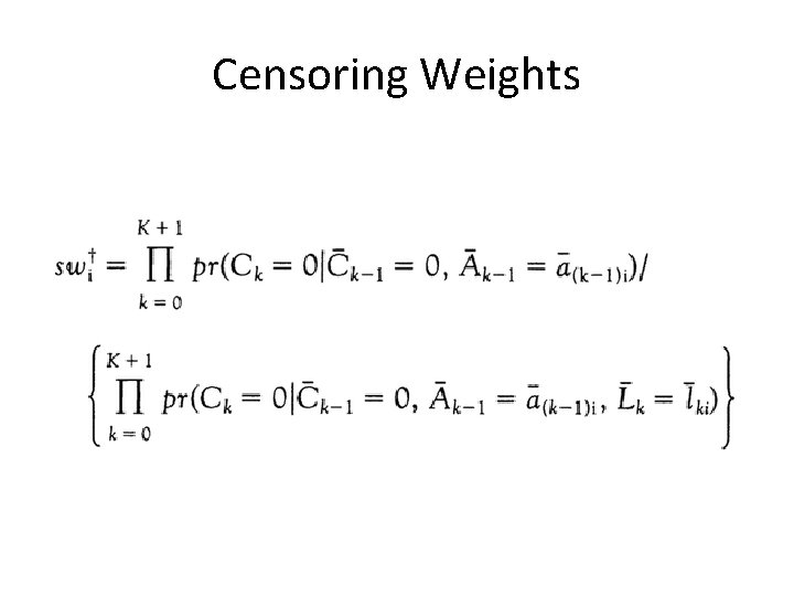
Censoring Weights

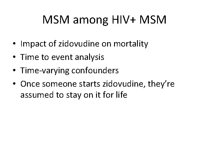
MSM among HIV+ MSM • • Impact of zidovudine on mortality Time to event analysis Time-varying confounders Once someone starts zidovudine, they’re assumed to stay on it for life

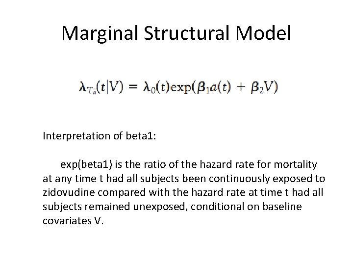
Marginal Structural Model Interpretation of beta 1: exp(beta 1) is the ratio of the hazard rate for mortality at any time t had all subjects been continuously exposed to zidovudine compared with the hazard rate at time t had all subjects remained unexposed, conditional on baseline covariates V.

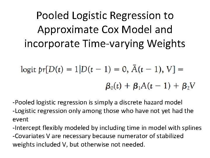
Pooled Logistic Regression to Approximate Cox Model and incorporate Time-varying Weights -Pooled logistic regression is simply a discrete hazard model -Logistic regression only among those who have not yet had the event -Intercept flexibly modeled by including time in model with splines -Covariates V are necessary because numerator of stabilized weights included V, but otherwise not needed.

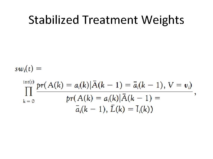
Stabilized Treatment Weights

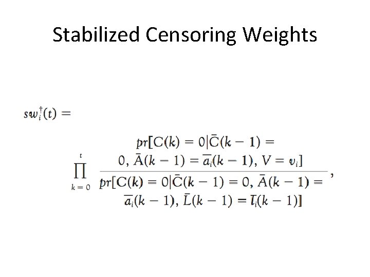
Stabilized Censoring Weights

In practice • Usually requires breaking up time into discrete intervals (e. g. , months or 3 -month periods). • Observations are often not measured at each interval, so may require some imputation or last observations carried forward. • Data prep is usually the most time-consuming part. • Within each interval, fit 2 (pooled) logistic regression models for the probability of starting treatment over time – using baseline covariates only (or not) [numerator of SW] – Using baseline and time-varying covariates [denom of SW]

In practice (2) • Within each interval, fit 2 pooled logistic regression models for the probability of being censored – using baseline covariates only (or not) – Using baseline and time-varying covariates • Compute predicted probability of patient following treatment history they followed thru time t – Using baseline covariates – Using baseline and time-varying covariates • Compute predicted probability of patient not being censored by time t – Using baseline covariates – Using baseline and time-varying covariates

In practice (3) • Multiply probabilities together to create time-varying inverse probability weights. • Weights may need to be windsorized (truncated) if extreme. • Fit a pooled logistic regression model using timevarying weights. • Time included in the model using flexible functions (e. g. , splines) • Variances are estimated using robust standard errors – i. e. , GEE with independence working covariance matrices