Marginal structural models for differential attrition timevarying exposures

Marginal structural models for differential attrition , time-varying exposures, and time-dependent confounding Another talk Jennifer Weuve, MPH, Sc. D jweuve@bu. edu http: //jweuve. tumblr. com/

Objectives (primary) • Define selection bias in the context of causal questions embedded in longitudinal studies • Explain why conventional methods fail when differential selection is present

Objectives (primary) • Work through the logic of: – What inverse probability-ofcontinuation weights (IPCW) encode – How using them can correct bias from differential selection • Explore the major steps of applying IPCW using real-life examples

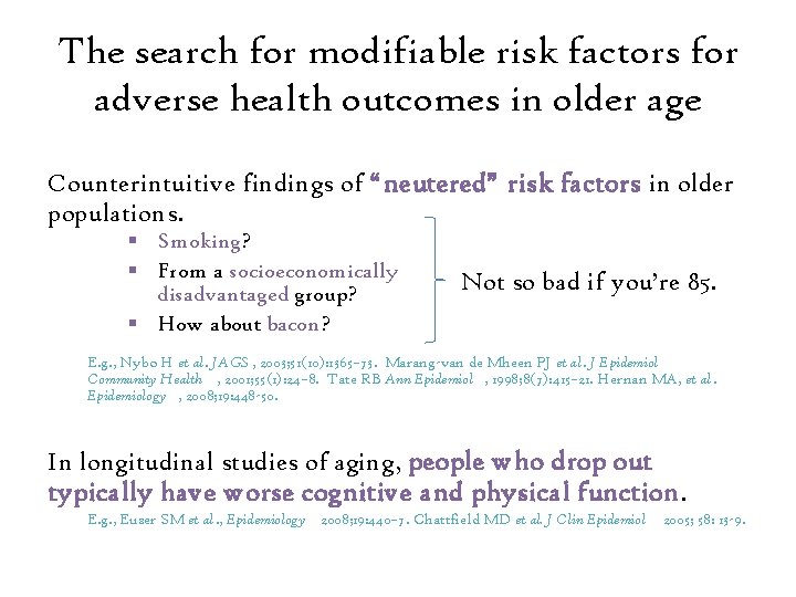
The search for modifiable risk factors for adverse health outcomes in older age Counterintuitive findings of “neutered” risk factors in older populations. § Smoking? § From a socioeconomically disadvantaged group? § How about bacon? Not so bad if you’re 85. E. g. , Nybo H et al. JAGS , 2003; 51(10): 1365– 73. Marang-van de Mheen PJ et al. J Epidemiol Community Health , 2001; 55(1): 24– 8. Tate RB Ann Epidemiol , 1998; 8(7): 415– 21. Hernan MA, et al. Epidemiology , 2008; 19: 448 -50. In longitudinal studies of aging, people who drop out typically have worse cognitive and physical function. E. g. , Euser SM et al. , Epidemiology 2008; 19: 440– 7. Chattfield MD et al. J Clin Epidemiol 2005; 58: 13 -9.

Example 1 Does cigarette smoking hasten cognitive decline?

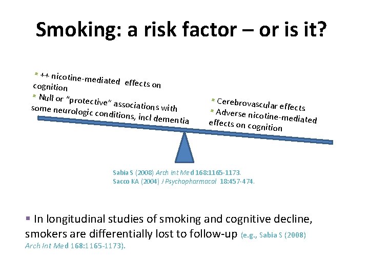
Smoking: a risk factor – or is it? § ++ nicotine-m ediated effect s on cognition § Null or “prote ctive” associat ions with some neurolog ic conditions, in cl dementia § Cerebrovascu lar effects § Adverse nico tine-mediated effects on cogn ition Sabia S (2008) Arch Int Med 168: 1165 -1173. Sacco KA (2004) J Psychopharmacol 18: 457 -474. § In longitudinal studies of smoking and cognitive decline, smokers are differentially lost to follow-up (e. g. , Sabia S (2008) Arch Int Med 168: 1165 -1173).

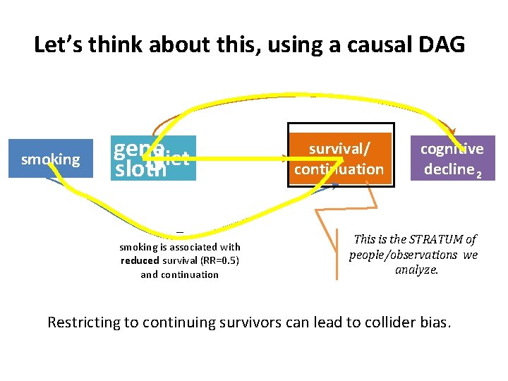
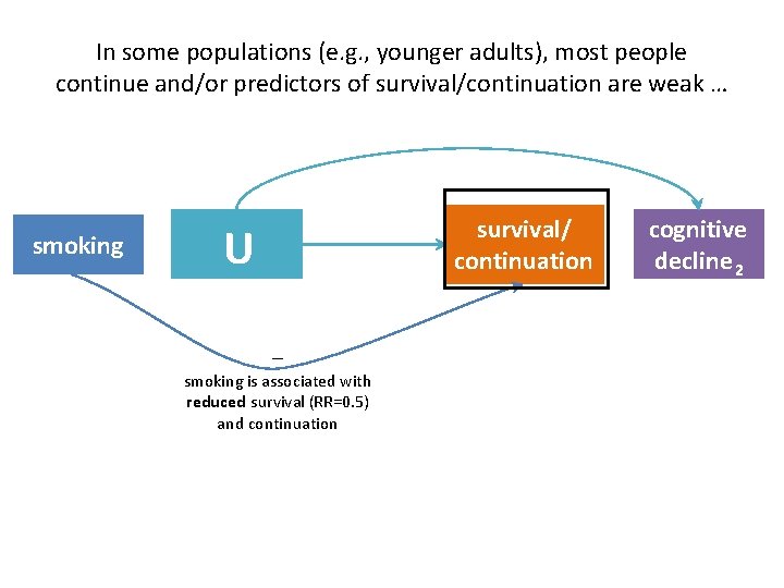
Let’s think about this, using a causal DAG smoking genediet U sloth – smoking is associated with reduced survival (RR=0. 5) and continuation survival/ continuation cognitive decline 2 This is the STRATUM of people/observations we analyze. Restricting to continuing survivors can lead to collider bias.

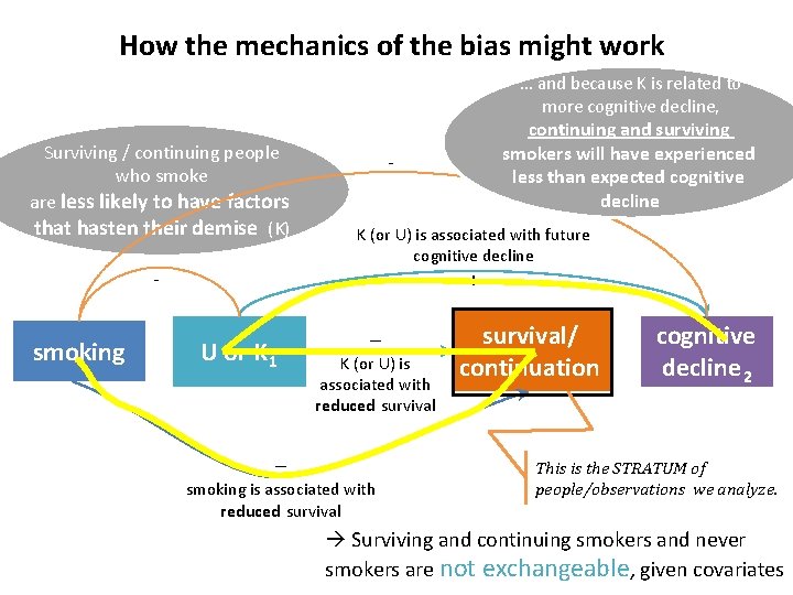
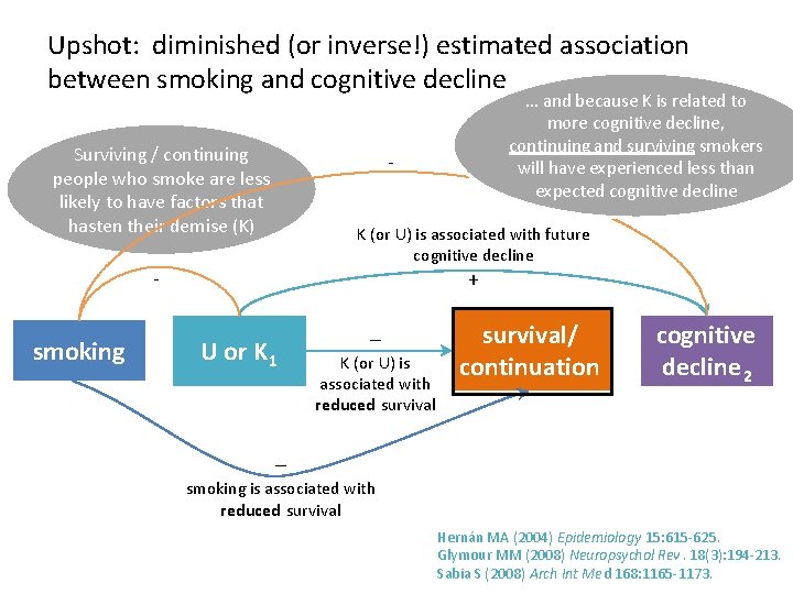
How the mechanics of the bias might work … and because K is related to more cognitive decline, Surviving / continuing people who smoke are less likely to have factors that hasten their demise (K) - K (or U) is associated with future cognitive decline + - smoking continuing and surviving smokers will have experienced less than expected cognitive decline U or K 1 – – K (or U) is associated with reduced survival smoking is associated with reduced survival/ continuation cognitive decline 2 This is the STRATUM of people/observations we analyze. Surviving and continuing smokers and never smokers are not exchangeable, given covariates

In some populations (e. g. , younger adults), most people continue and/or predictors of survival/continuation are weak … smoking survival/ continuation U – smoking is associated with reduced survival (RR=0. 5) and continuation cognitive decline 2

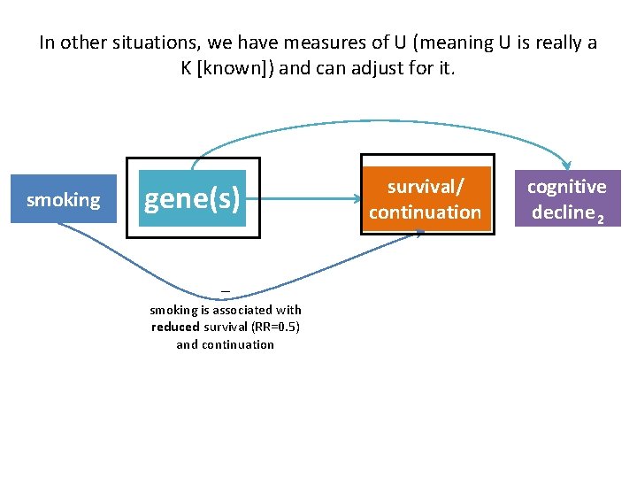
In other situations, we have measures of U (meaning U is really a K [known]) and can adjust for it. smoking gene(s) – smoking is associated with reduced survival (RR=0. 5) and continuation survival/ continuation cognitive decline 2

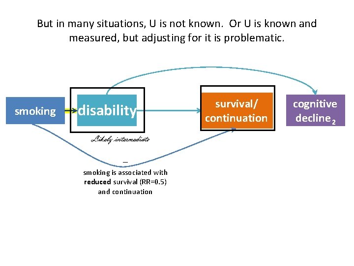
But in many situations, U is not known. Or U is known and measured, but adjusting for it is problematic. smoking disability Likely intermediate – smoking is associated with reduced survival (RR=0. 5) and continuation survival/ continuation cognitive decline 2

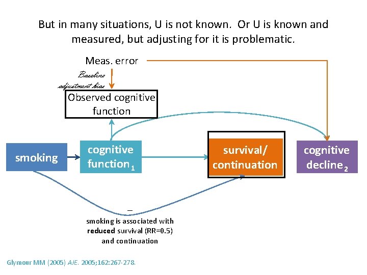
But in many situations, U is not known. Or U is known and measured, but adjusting for it is problematic. Meas. error Baseline adjustment bias Observed cognitive function smoking cognitive function 1 – smoking is associated with reduced survival (RR=0. 5) and continuation Glymour MM (2005) AJE. 2005; 162: 267 -278. survival/ continuation cognitive decline 2

Upshot: diminished (or inverse!) estimated association between smoking and cognitive decline Surviving / continuing people who smoke are less likely to have factors that hasten their demise (K) - K (or U) is associated with future cognitive decline + - smoking … and because K is related to more cognitive decline, continuing and surviving smokers will have experienced less than expected cognitive decline U or K 1 – K (or U) is associated with reduced survival/ continuation cognitive decline 2 – smoking is associated with reduced survival Hernán MA (2004) Epidemiology 15: 615 -625. Glymour MM (2008) Neuropsychol Rev. 18(3): 194 -213. Sabia S (2008) Arch Int Med 168: 1165 -1173.

Example 2 Does exposure to air pollution hasten decline in physical function?

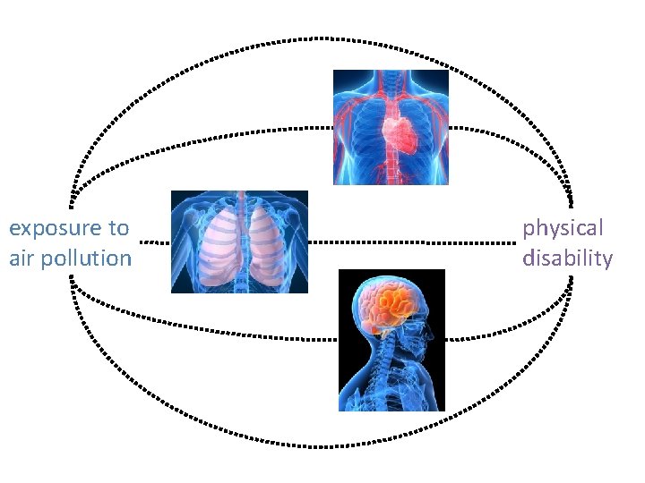
exposure to air pollution physical disability

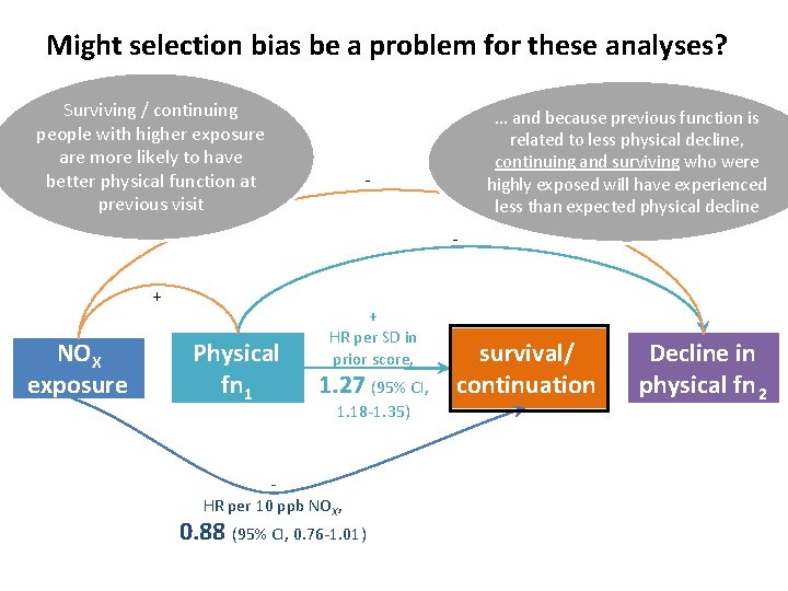
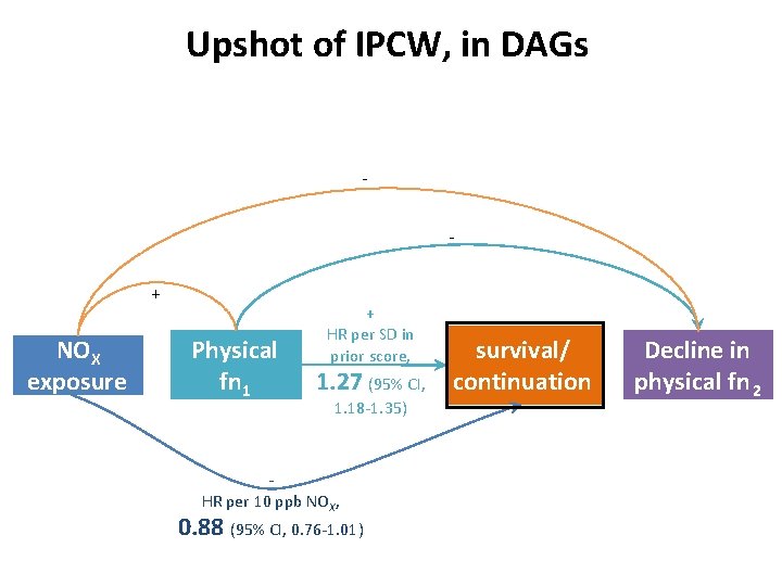
Might selection bias be a problem for these analyses? Surviving / continuing people with higher exposure are more likely to have better physical function at previous visit … and because previous function is related to less physical decline, continuing and surviving who were highly exposed will have experienced less than expected physical decline - + NOX exposure Physical fn 1 + HR per SD in prior score, 1. 27 (95% CI, 1. 18 -1. 35) HR per 10 ppb NOX, 0. 88 (95% CI, 0. 76 -1. 01) survival/ continuation Decline in physical fn 2

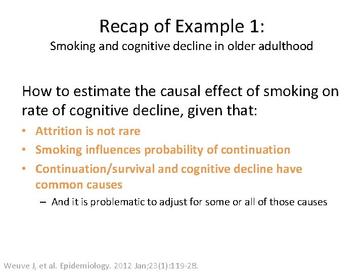
Recap of Example 1: Smoking and cognitive decline in older adulthood How to estimate the causal effect of smoking on rate of cognitive decline, given that: • Attrition is not rare • Smoking influences probability of continuation • Continuation/survival and cognitive decline have common causes – And it is problematic to adjust for some or all of those causes Weuve J, et al. Epidemiology. 2012 Jan; 23(1): 119 -28.

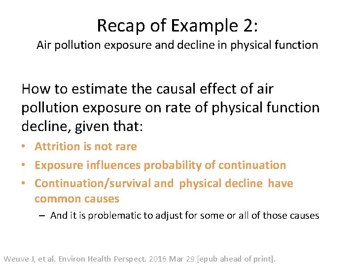
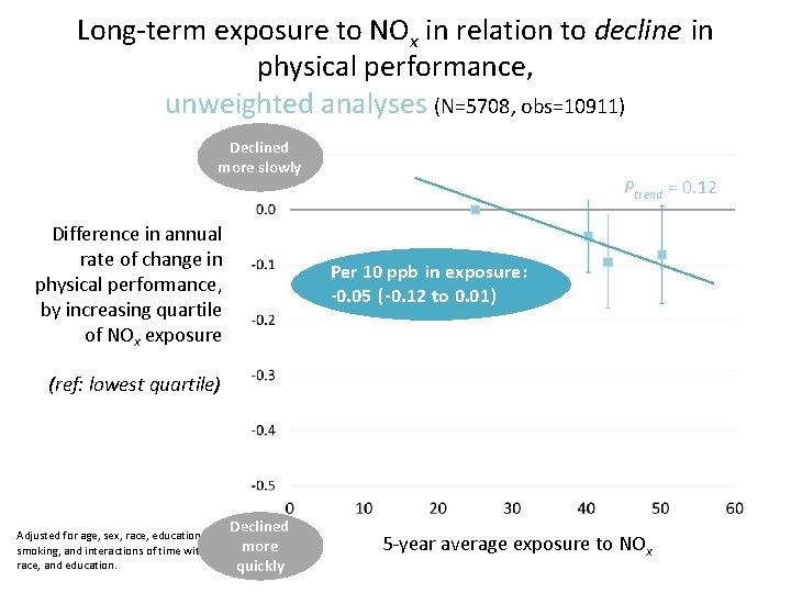
Recap of Example 2: Air pollution exposure and decline in physical function How to estimate the causal effect of air pollution exposure on rate of physical function decline, given that: • Attrition is not rare • Exposure influences probability of continuation • Continuation/survival and physical decline have common causes – And it is problematic to adjust for some or all of those causes Weuve J, et al. Environ Health Perspect. 2016 Mar 29 [epub ahead of print].

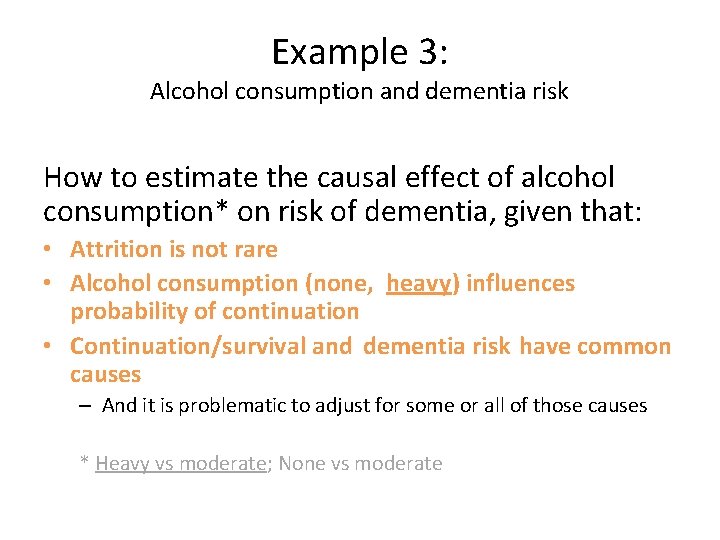
Example 3: Alcohol consumption and dementia risk How to estimate the causal effect of alcohol consumption* on risk of dementia, given that: • Attrition is not rare • Alcohol consumption (none, heavy) influences probability of continuation • Continuation/survival and dementia risk have common causes – And it is problematic to adjust for some or all of those causes * Heavy vs moderate; None vs moderate

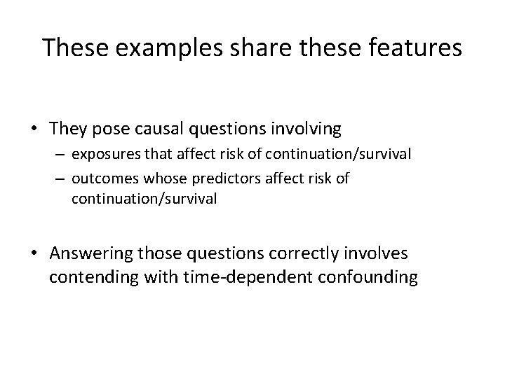
These examples share these features • They pose causal questions involving – exposures that affect risk of continuation/survival – outcomes whose predictors affect risk of continuation/survival • Answering those questions correctly involves contending with time-dependent confounding

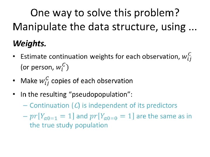
One way to solve this problem? Manipulate the data structure, using. . . •

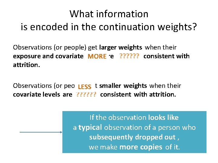
What information is encoded in the continuation weights? Observations (or people) get larger weights when their exposure and covariate levels MOREare ? ? ? consistent with attrition. Observations (or people) get smaller weights when their LESS covariate levels are ? ? ? consistent with attrition. If the observation looks like a typical observation of a person who subsequently dropped out , we make more copies of it.

Upshot of IPCW, in DAGs + NOX exposure Physical fn 1 + HR per SD in prior score, 1. 27 (95% CI, 1. 18 -1. 35) HR per 10 ppb NOX, 0. 88 (95% CI, 0. 76 -1. 01) survival/ continuation Decline in physical fn 2

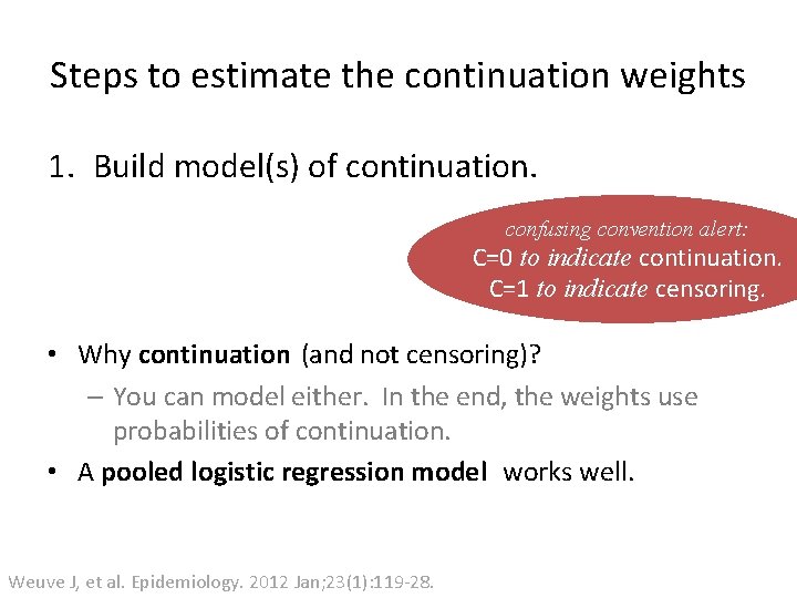
Steps to estimate the continuation weights 1. Build model(s) of continuation. confusing convention alert: C=0 to indicate continuation. C=1 to indicate censoring. • Why continuation (and not censoring)? – You can model either. In the end, the weights use probabilities of continuation. • A pooled logistic regression model works well. Weuve J, et al. Epidemiology. 2012 Jan; 23(1): 119 -28.

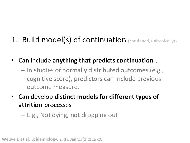
1. Build model(s) of continuation (continued, unironically). • Can include anything that predicts continuation. – In studies of normally distributed outcomes (e. g. , cognitive score), predictors can include previous outcome measure. • Can develop distinct models for different types of attrition processes – E. g. , Not dying, not dropping out Weuve J, et al. Epidemiology. 2012 Jan; 23(1): 119 -28.

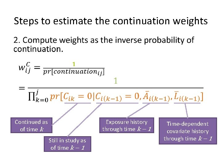
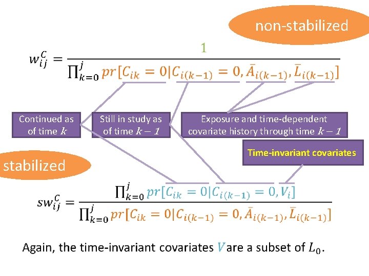
Steps to estimate the continuation weights • Continued as of time k Still in study as of time k − 1 Exposure history through time k − 1 Time-dependent covariate history through time k − 1

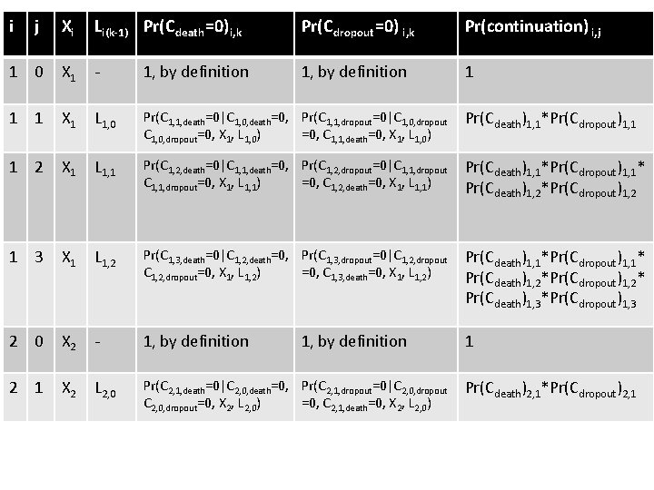
i j Xi Li(k-1) Pr(C death =0) i, k Pr(C dropout =0) i, k Pr(continuation) i, j 1 0 X 1 - 1, by definition 1 1 1 X 1 L 1, 0 Pr(C 1, 1, death=0|C 1, 0, death=0, Pr(C 1, 1, dropout=0|C 1, 0, dropout=0, X 1, L 1, 0) =0, C 1, 1, death=0, X 1, L 1, 0) Pr(Cdeath)1, 1*Pr(Cdropout)1, 1 1 2 X 1 L 1, 1 Pr(C 1, 2, death=0|C 1, 1, death=0, Pr(C 1, 2, dropout=0|C 1, 1, dropout=0, X 1, L 1, 1) =0, C 1, 2, death=0, X 1, L 1, 1) Pr(Cdeath)1, 1*Pr(Cdropout)1, 1* Pr(Cdeath)1, 2*Pr(Cdropout)1, 2 1 3 X 1 L 1, 2 Pr(C 1, 3, death=0|C 1, 2, death=0, Pr(C 1, 3, dropout=0|C 1, 2, dropout=0, X 1, L 1, 2) =0, C 1, 3, death=0, X 1, L 1, 2) Pr(Cdeath)1, 1*Pr(Cdropout)1, 1* Pr(Cdeath)1, 2*Pr(Cdropout)1, 2* Pr(Cdeath)1, 3*Pr(Cdropout)1, 3 2 0 X 2 - 1, by definition 1 2 1 X 2 L 2, 0 Pr(C 2, 1, death=0|C 2, 0, death=0, Pr(C 2, 1, dropout=0|C 2, 0, dropout=0, X 2, L 2, 0) =0, C 2, 1, death=0, X 2, L 2, 0) 1, by definition Pr(Cdeath)2, 1*Pr(Cdropout)2, 1

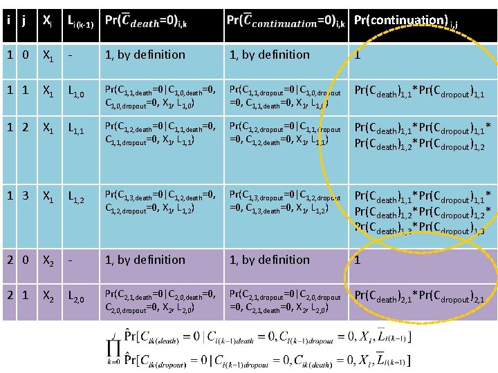
i j Xi Li(k-1) Pr(continuation) i, j 1 0 X 1 - 1, by definition 1 1 X 1 L 1, 0 Pr(C 1, 1, death=0|C 1, 0, death=0, Pr(C 1, 1, dropout=0|C 1, 0, dropout=0, X 1, L 1, 0) =0, C 1, 1, death=0, X 1, L 1, 0) Pr(Cdeath)1, 1*Pr(Cdropout)1, 1 1 2 X 1 L 1, 1 Pr(C 1, 2, death=0|C 1, 1, death=0, Pr(C 1, 2, dropout=0|C 1, 1, dropout=0, X 1, L 1, 1) =0, C 1, 2, death=0, X 1, L 1, 1) Pr(Cdeath)1, 1*Pr(Cdropout)1, 1* Pr(Cdeath)1, 2*Pr(Cdropout)1, 2 1 3 X 1 L 1, 2 Pr(C 1, 3, death=0|C 1, 2, death=0, Pr(C 1, 3, dropout=0|C 1, 2, dropout=0, X 1, L 1, 2) =0, C 1, 3, death=0, X 1, L 1, 2) Pr(Cdeath)1, 1*Pr(Cdropout)1, 1* Pr(Cdeath)1, 2*Pr(Cdropout)1, 2* Pr(Cdeath)1, 3*Pr(Cdropout)1, 3 2 0 X 2 - 1, by definition 1 2 1 X 2 L 2, 0 Pr(C 2, 1, death=0|C 2, 0, death=0, Pr(C 2, 1, dropout=0|C 2, 0, dropout=0, X 2, L 2, 0) =0, C 2, 1, death=0, X 2, L 2, 0) 1, by definition 1 Pr(Cdeath)2, 1*Pr(Cdropout)2, 1

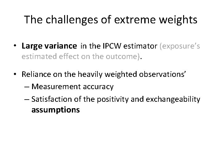
The challenges of extreme weights • Large variance in the IPCW estimator (exposure’s estimated effect on the outcome). • Reliance on the heavily weighted observations’ – Measurement accuracy – Satisfaction of the positivity and exchangeability assumptions

One solution: stabilize the weights by altering the numerator

non-stabilized • Continued as of time k stabilized Still in study as of time k − 1 Exposure and time-dependent covariate history through time k − 1 Time-invariant covariates

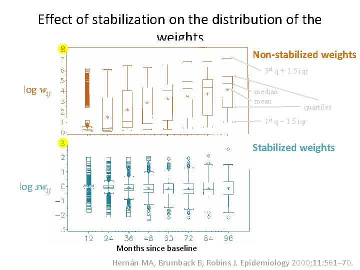
Effect of stabilization on the distribution of the weights 8 Non-stabilized weights 3 rd q + 1. 5 iqr log wij median mean quartiles 1 st q ‒ 1. 5 iqr 3 Stabilized weights log swij Months since baseline Hernán MA, Brumback B, Robins J. Epidemiology 2000; 11: 561– 70.

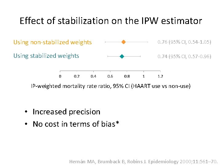
Effect of stabilization on the IPW estimator Using non-stabilized weights 0. 76 (95% CI, 0. 54 -1. 05) Using stabilized weights 0. 74 (95% CI, 0. 57 -0. 96) IP-weighted mortality rate ratio, 95% CI (HAART use vs non-use) • Increased precision • No cost in terms of bias* Hernán MA, Brumback B, Robins J. Epidemiology 2000; 11: 561– 70.

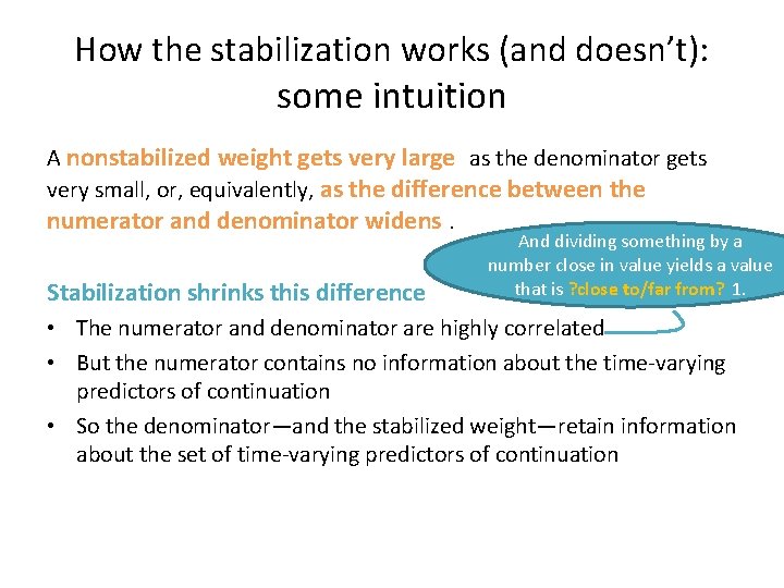
How the stabilization works (and doesn’t): some intuition A nonstabilized weight gets very large as the denominator gets very small, or, equivalently, as the difference between the numerator and denominator widens. Stabilization shrinks this difference And dividing something by a number close in value yields a value that is ? close to/far from? 1. • The numerator and denominator are highly correlated • But the numerator contains no information about the time-varying predictors of continuation • So the denominator—and the stabilized weight—retain information about the set of time-varying predictors of continuation

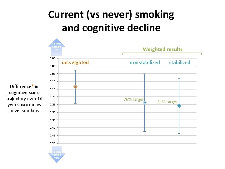
So? Results from unweighted analyses and analyses weighted by IPCWs

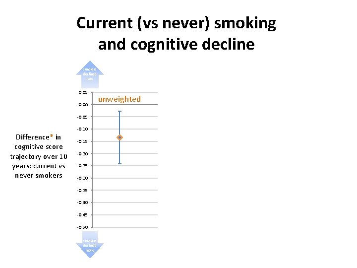
Current (vs never) smoking and cognitive decline smokers declined less 0. 05 0. 00 Weighted results unweighted nonstabilized -0. 05 Difference* in cognitive score trajectory over 10 years: current vs never smokers -0. 10 -0. 15 -0. 20 -0. 25 -0. 30 -0. 35 -0. 40 -0. 45 -0. 50 smokers declined more 56% larger 86% larger

Current (vs never) smoking and cognitive decline smokers declined less 0. 05 0. 00 Weighted results unweighted nonstabilized -0. 05 Difference* in cognitive score trajectory over 10 years: current vs never smokers -0. 10 -0. 15 -0. 20 -0. 25 -0. 30 -0. 35 -0. 40 -0. 45 -0. 50 smokers declined more 76% larger 91% larger

Long-term exposure to NOx in relation to decline in physical performance, unweighted analyses (N=5708, obs=10911) Declined more slowly Difference in annual rate of change in physical performance, by increasing quartile of NOx exposure Ptrend = 0. 12 Per 10 ppb in exposure: -0. 05 (-0. 12 to 0. 01) (ref: lowest quartile) Declined Adjusted for age, sex, race, education, income, more smoking, and interactions of time with age, sex, race, and education. quickly 5 -year average exposure to NOx

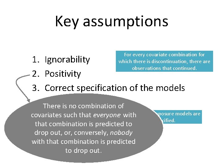
Key assumptions For every covariate combination for which there is discontinuation, there are observations that continued. 1. Ignorability 2. Positivity 3. Correct specification of the models There is no combination of Both structural and exposure models are covariates such that everyone with correctly specified. that combination is predicted to drop out, or, conversely, nobody with that combination is predicted to drop out.

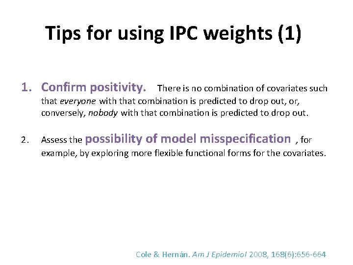
Tips for using IPC weights (1) 1. Confirm positivity. There is no combination of covariates such that everyone with that combination is predicted to drop out, or, conversely, nobody with that combination is predicted to drop out. 2. Assess the possibility of model misspecification , for example, by exploring more flexible functional forms for the covariates. Cole & Hernán. Am J Epidemiol 2008, 168(6): 656 -664

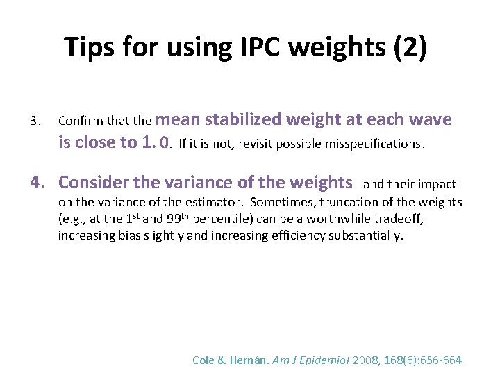
Tips for using IPC weights (2) 3. Confirm that the mean stabilized weight at each wave is close to 1. 0. If it is not, revisit possible misspecifications. 4. Consider the variance of the weights and their impact on the variance of the estimator. Sometimes, truncation of the weights (e. g. , at the 1 st and 99 th percentile) can be a worthwhile tradeoff, increasing bias slightly and increasing efficiency substantially. Cole & Hernán. Am J Epidemiol 2008, 168(6): 656 -664

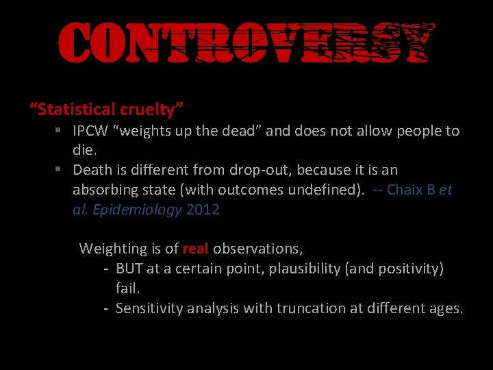
CONTROVERSY “Statistical cruelty” § IPCW “weights up the dead” and does not allow people to die. § Death is different from drop-out, because it is an absorbing state (with outcomes undefined). -- Chaix B et al. Epidemiology 2012 Weighting is of real observations, - BUT at a certain point, plausibility (and positivity) fail. - Sensitivity analysis with truncation at different ages.

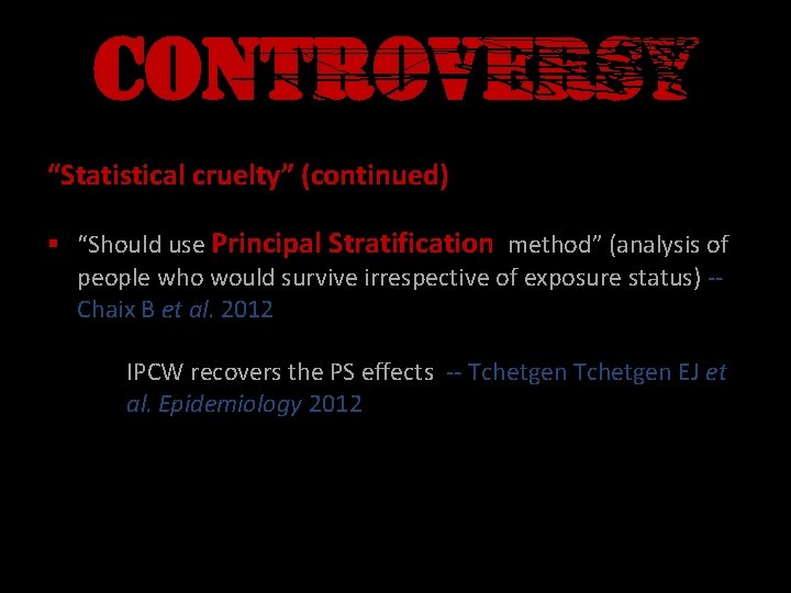
CONTROVERSY “Statistical cruelty” (continued) § “Should use Principal Stratification method” (analysis of people who would survive irrespective of exposure status) -- Chaix B et al. 2012 IPCW recovers the PS effects -- Tchetgen EJ et al. Epidemiology 2012

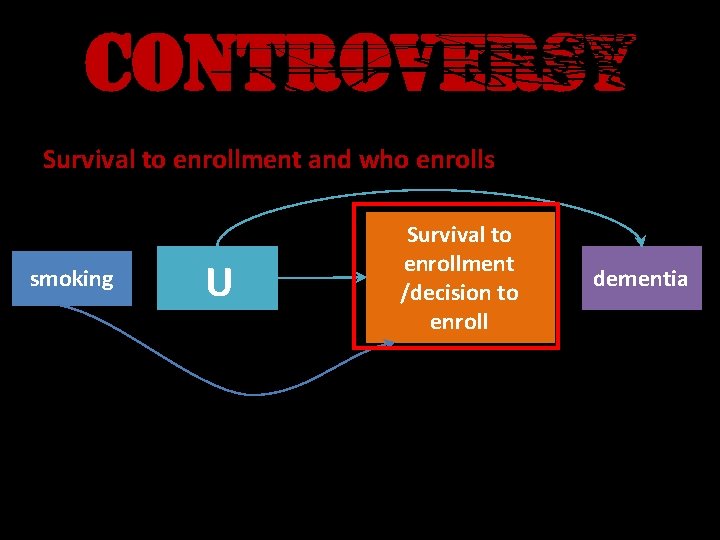
CONTROVERSY Survival to enrollment and who enrolls smoking Survival to enrollment /decision to enroll U – smoking is associated with reduced survival (RR=0. 5) and continuation dementia

Objectives (as needed) • Explore the types of causal questions embedded in “time-varying exposures” • Define the conditions underlying time- dependent confounding • Explain why conventional methods fail when time-depending confounding is present

Objectives (as needed) • Work through the logic of: – What inverse probability-of-treatment weights (IPTW) encode – How using them can correct bias from timedependent confounding • Explore the major steps of applying IPTW using several real-life examples

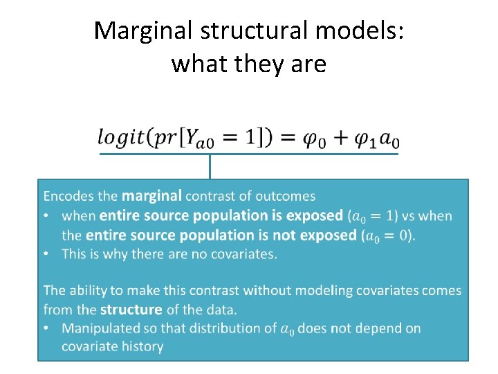
Marginal structural models: what they are •