Mar 3 More Iterative Methods Iterative Refinement nonpolynomial

Mar 3: More Iterative Methods • Iterative Refinement (non-polynomial view) • Polynomial method • Chebyshev Iteration

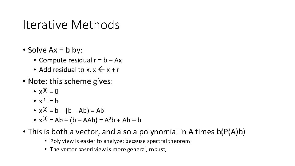
Iterative Methods • Solve Ax = b by: • Compute residual r = b – Ax • Add residual to x, x x + r • Note: this scheme gives: • • x(0) = 0 x(1) = b x(2) = b – (b – Ab) = Ab x(3) = Ab – (b – AAb) = A 2 b + Ab – b • This is both a vector, and also a polynomial in A times b(P(A)b) • Poly view is easier to analyze: because spectral theorem • The vector based view is more general, robust,

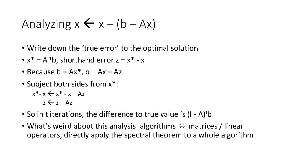
Analyzing x x + (b – Ax) • Write down the ‘true error’ to the optimal solution • x* = A-1 b, shorthand error z = x* - x • Because b = Ax*, b – Ax = Az • Subject both sides from x*: x*- x x* - x – Az z z – Az • So in t iterations, the difference to true value is (I - A)tb • What’s weird about this analysis: algorithms matrices / linear operators, directly apply the spectral theorem to a whole algorithm

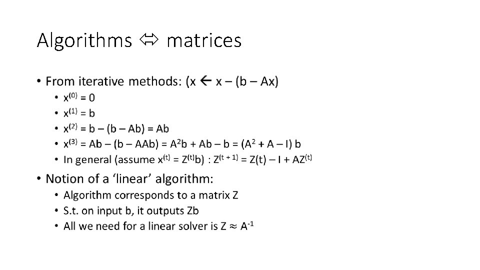
Algorithms matrices •

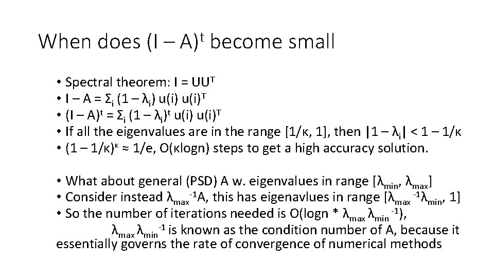
When does (I – A)t become small • Spectral theorem: I = UUT • I – A = Σi (1 – λi) u(i)T • (I – A)t = Σi (1 – λi)t u(i)T • If all the eigenvalues are in the range [1/κ, 1], then |1 – λi| < 1 – 1/κ • (1 – 1/κ)κ ≈ 1/e, O(κlogn) steps to get a high accuracy solution. • What about general (PSD) A w. eigenvalues in range [λmin, λmax] • Consider instead λmax-1 A, this has eigenavlues in range [λmax -1λmin, 1] • So the number of iterations needed is O(logn * λmax λmin -1), λmax λmin-1 is known as the condition number of A, because it essentially governs the rate of convergence of numerical methods

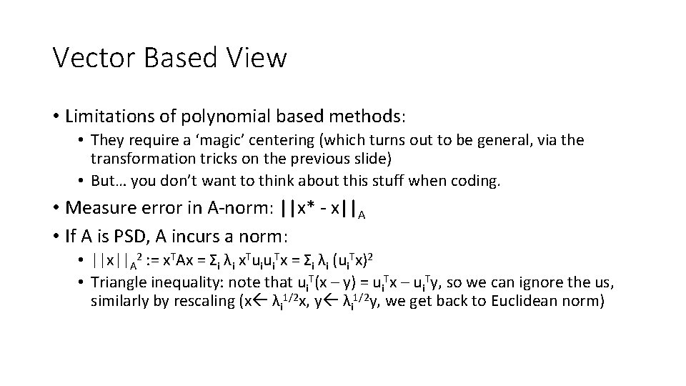
Vector Based View • Limitations of polynomial based methods: • They require a ‘magic’ centering (which turns out to be general, via the transformation tricks on the previous slide) • But… you don’t want to think about this stuff when coding. • Measure error in A-norm: ||x* - x||A • If A is PSD, A incurs a norm: • ||x||A 2 : = x. TAx = Σi λi x. Tuiui. Tx = Σi λi (ui. Tx)2 • Triangle inequality: note that ui. T(x – y) = ui. Tx – ui. Ty, so we can ignore the us, similarly by rescaling (x λi 1/2 x, y λi 1/2 y, we get back to Euclidean norm)

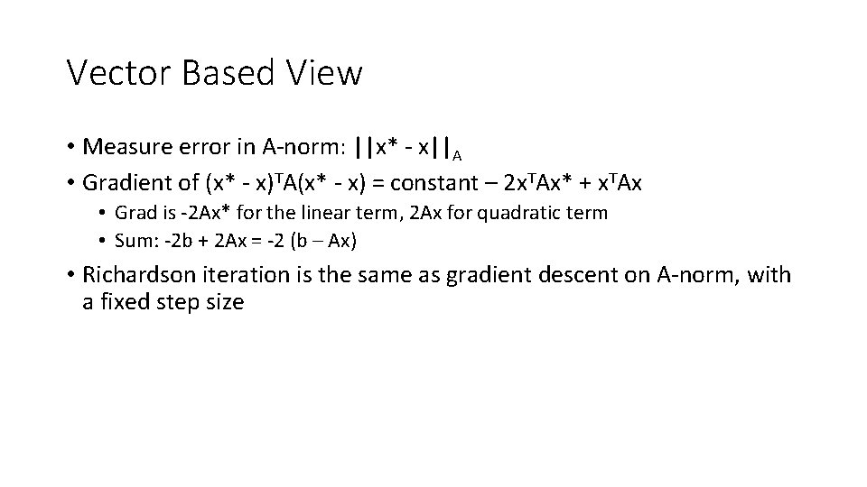
Vector Based View • Measure error in A-norm: ||x* - x||A • Gradient of (x* - x)TA(x* - x) = constant – 2 x. TAx* + x. TAx • Grad is -2 Ax* for the linear term, 2 Ax for quadratic term • Sum: -2 b + 2 Ax = -2 (b – Ax) • Richardson iteration is the same as gradient descent on A-norm, with a fixed step size

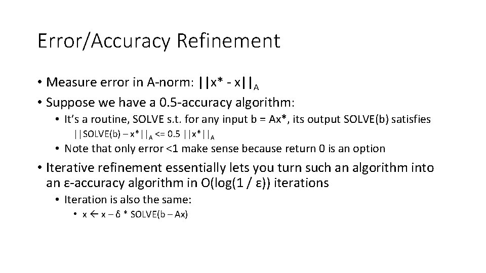
Error/Accuracy Refinement • Measure error in A-norm: ||x* - x||A • Suppose we have a 0. 5 -accuracy algorithm: • It’s a routine, SOLVE s. t. for any input b = Ax*, its output SOLVE(b) satisfies ||SOLVE(b) – x*||A <= 0. 5 ||x*||A • Note that only error <1 make sense because return 0 is an option • Iterative refinement essentially lets you turn such an algorithm into an ε-accuracy algorithm in O(log(1 / ε)) iterations • Iteration is also the same: • x x – δ * SOLVE(b – Ax)

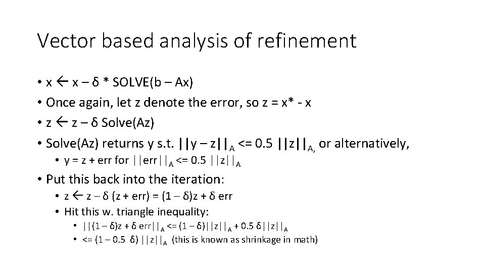
Vector based analysis of refinement • x x – δ * SOLVE(b – Ax) • Once again, let z denote the error, so z = x* - x • z z – δ Solve(Az) • Solve(Az) returns y s. t. ||y – z||A <= 0. 5 ||z||A, or alternatively, • y = z + err for ||err||A <= 0. 5 ||z||A • Put this back into the iteration: • z z – δ (z + err) = (1 – δ)z + δ err • Hit this w. triangle inequality: • ||(1 – δ)z + δ err||A <= (1 – δ)||z||A + 0. 5 δ||z||A • <= (1 – 0. 5 δ) ||z||A (this is known as shrinkage in math)

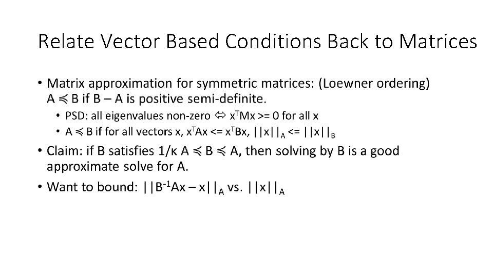
Relate Vector Based Conditions Back to Matrices •

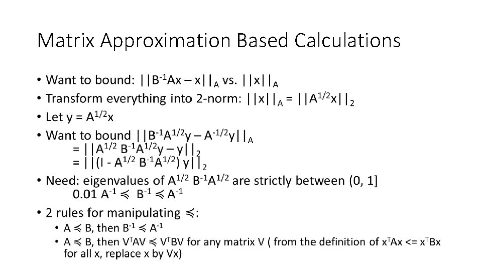
Matrix Approximation Based Calculations •

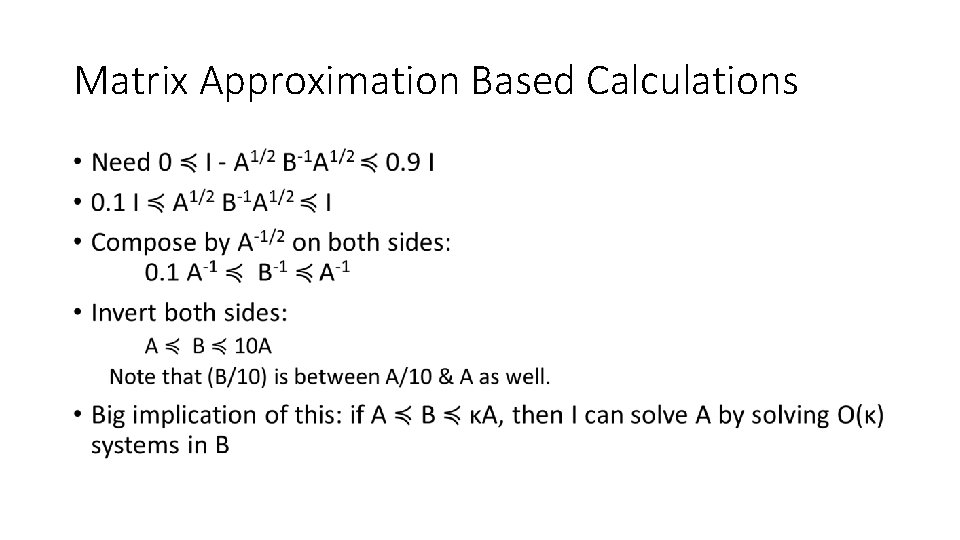
Matrix Approximation Based Calculations •

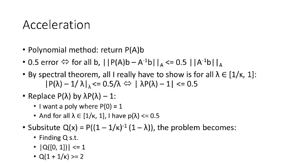
Acceleration •

Build Polynomial • Finding small degree Q s. t. • |Q([0, 1])| <= 1 • Q(1 + 1/κ) >= 2 • Richardson: Q(x) = xd for d = O(κ) • Chebyshev polynomial: cos dθ as a polynomial in cos θ • Think of θ = arccos x • cos dθ + i sin dθ = (cos θ + i sin θ )d • cos dθ = ½ ((cos θ + i sin θ )d - (cos θ - i sin θ )d = Σi binom{d}{2 i} (cos θ)d-2 i (isin θ)2 i • Then note that (isinθ)2 = - (sinθ)2 = (cosθ)2 – 1 • So Cheby is Σi binom{d}{2 i} (cos θ)d-2 i ((cosθ)2 – 1)i