Mar 22 IPM Linear Programming Central Path Path

Mar 22: IPM • Linear Programming & Central Path • Path Following Using L 2 minimization

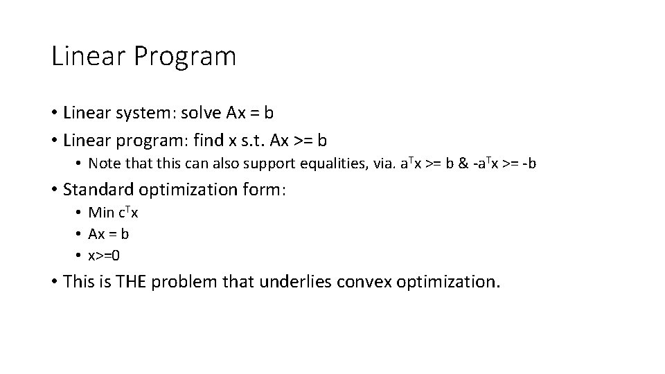
Linear Program • Linear system: solve Ax = b • Linear program: find x s. t. Ax >= b • Note that this can also support equalities, via. a. Tx >= b & -a. Tx >= -b • Standard optimization form: • Min c. Tx • Ax = b • x>=0 • This is THE problem that underlies convex optimization.

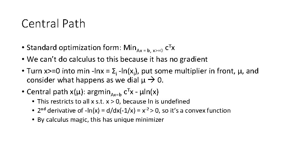
Central Path • Standard optimization form: Min. Ax = b, x>=0 c. Tx • We can’t do calculus to this because it has no gradient • Turn x>=0 into min -lnx = Σi -ln(xi), put some multiplier in front, μ, and consider what happens as we dial μ 0. • Central path x(μ): argmin. Ax=b c. Tx - μln(x) • This restricts to all x s. t. x > 0, because ln is undefined • 2 nd derivative of -ln(x) = d/dx(-1/x) = x-2 > 0, so it’s a convex function • By calculus magic, this has unique minimizer

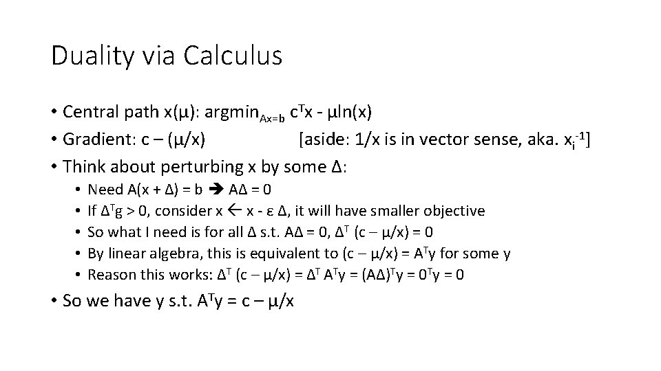
Duality via Calculus • Central path x(μ): argmin. Ax=b c. Tx - μln(x) • Gradient: c – (μ/x) [aside: 1/x is in vector sense, aka. xi-1] • Think about perturbing x by some Δ: • • • Need A(x + Δ) = b AΔ = 0 If ΔTg > 0, consider x x - ε Δ, it will have smaller objective So what I need is for all Δ s. t. AΔ = 0, ΔT (c – μ/x) = 0 By linear algebra, this is equivalent to (c – μ/x) = ATy for some y Reason this works: ΔT (c – μ/x) = ΔT ATy = (AΔ)Ty = 0 • So we have y s. t. ATy = c – μ/x

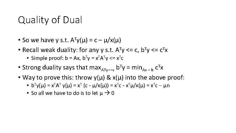
Quality of Dual • So we have y s. t. ATy(μ) = c – μ/x(μ) • Recall weak duality: for any y s. t. ATy <= c, b. Ty <= c. Tx • Simple proof: b = Ax, b. Ty = x. TATy <= x. Tc • Strong duality says that max. ATy<=c b. Ty = min. Ax = b c. Tx • Way to prove this: throw y(μ) & x(μ) into the above proof: • b. Ty(μ) = x. TAT y(μ) = x. T (c - μ/x(μ)) = x. Tc - x. Tμ/x(μ) = x. Tc – μn • So all we have to do is to let μ 0

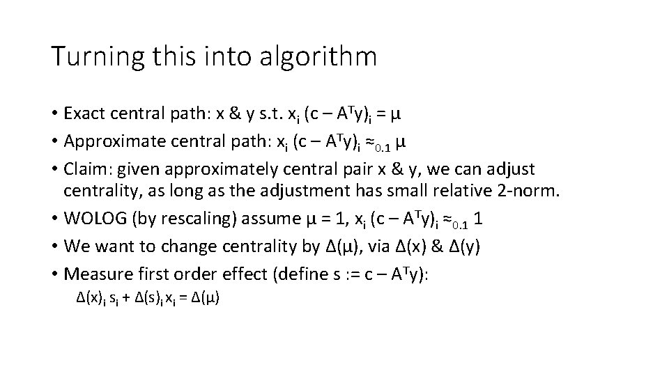
Turning this into algorithm • Exact central path: x & y s. t. xi (c – ATy)i = μ • Approximate central path: xi (c – ATy)i ≈0. 1 μ • Claim: given approximately central pair x & y, we can adjust centrality, as long as the adjustment has small relative 2 -norm. • WOLOG (by rescaling) assume μ = 1, xi (c – ATy)i ≈0. 1 1 • We want to change centrality by Δ(μ), via Δ(x) & Δ(y) • Measure first order effect (define s : = c – ATy): Δ(x)i si + Δ(s)i xi = Δ(μ)

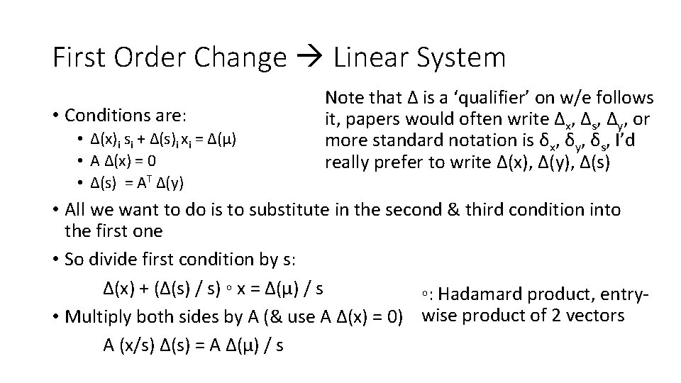
First Order Change Linear System • Conditions are: • Δ(x)i si + Δ(s)i xi = Δ(μ) • A Δ(x) = 0 • Δ(s) = AT Δ(y) Note that Δ is a ‘qualifier’ on w/e follows it, papers would often write Δx, Δs, Δy, or more standard notation is δx, δy, δs, I’d really prefer to write Δ(x), Δ(y), Δ(s) • All we want to do is to substitute in the second & third condition into the first one • So divide first condition by s: Δ(x) + (Δ(s) / s) ◦ x = Δ(μ) / s ◦: Hadamard product, entry • Multiply both sides by A (& use A Δ(x) = 0) wise product of 2 vectors A (x/s) Δ(s) = A Δ(μ) / s

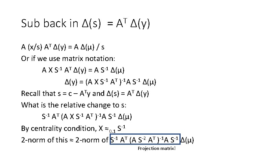
Sub back in Δ(s) = AT Δ(y) A (x/s) AT Δ(y) = A Δ(μ) / s Or if we use matrix notation: A X S-1 AT Δ(y) = A S-1 Δ(μ) Δ(y) = (A X S-1 AT )-1 A S-1 Δ(μ) Recall that s = c – ATy and Δ(s) = AT Δ(y) What is the relative change to s: S-1 AT (A X S-1 AT )-1 A S-1 Δ(μ) By centrality condition, X ≈0. 1 S-1 2 -norm of this ≈ 2 -norm of S-1 AT (A S-2 AT )-1 A S-1 Δ(μ) Projection matrix!

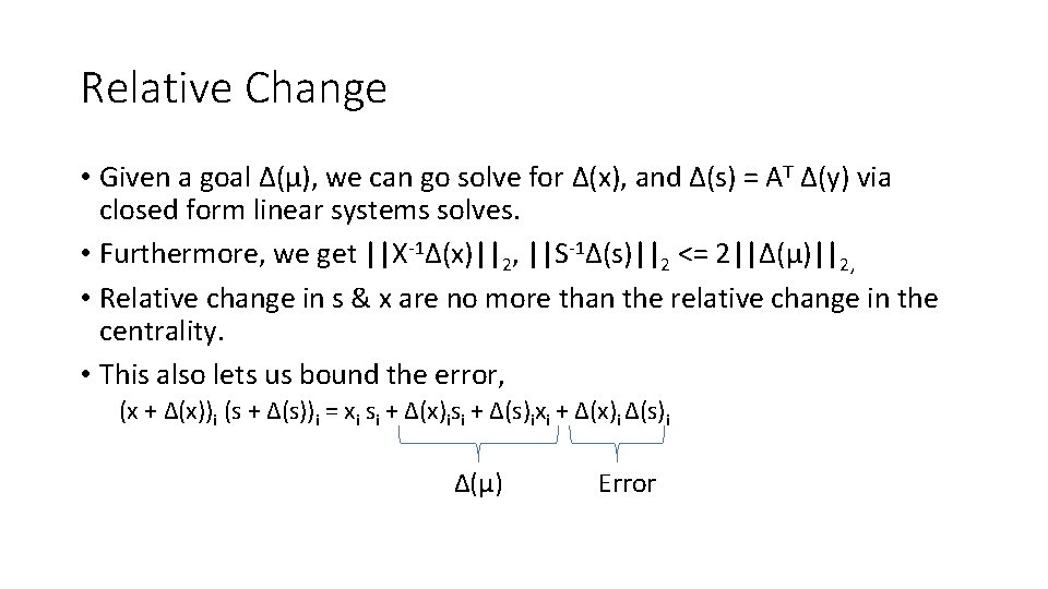
Relative Change • Given a goal Δ(μ), we can go solve for Δ(x), and Δ(s) = AT Δ(y) via closed form linear systems solves. • Furthermore, we get ||X-1Δ(x)||2, ||S-1Δ(s)||2 <= 2||Δ(μ)||2, • Relative change in s & x are no more than the relative change in the centrality. • This also lets us bound the error, (x + Δ(x))i (s + Δ(s))i = xi si + Δ(x)isi + Δ(s)ixi + Δ(x)i Δ(s)i Δ(μ) Error

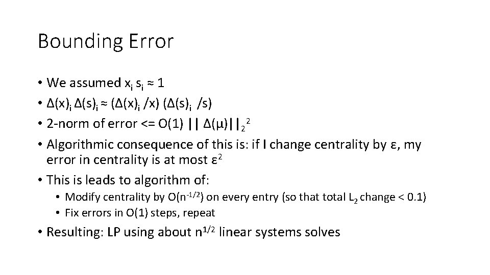
Bounding Error • We assumed xi si ≈ 1 • Δ(x)i Δ(s)i ≈ (Δ(x)i /x) (Δ(s)i /s) • 2 -norm of error <= O(1) || Δ(μ)||22 • Algorithmic consequence of this is: if I change centrality by ε, my error in centrality is at most ε 2 • This is leads to algorithm of: • Modify centrality by O(n-1/2) on every entry (so that total L 2 change < 0. 1) • Fix errors in O(1) steps, repeat • Resulting: LP using about n 1/2 linear systems solves