Mapping the Friction Coefficient of Asphalt Roads Using

Mapping the Friction Coefficient of Asphalt Roads Using Airborne Imaging Spectroscopy Nimrod Carmon and Eyal Ben-Dor* Porter School of Environmental and Erath Science Faculty of Exact Science Tel Aviv University, Tel Aviv, Israel *Correspondence: bendor@post. tau. ac. il

Outline • Friction coefficient and asphalt roads – Tradition Measurements • Spectral ground measurements: Proof of concept for optical HSR sensors • Optical HSR Airborne measurements: Road mapping • Spectral ground measurements: Proof of concept for thermal hsr sensors • Thermal HSR Airborne measurements: Road mapping • Future Ideas

Asphalt Composition “composite material composed of mineral aggregate adhered with a binder” • • • Micro and Macro textures which creates high friction with the rubber tire The binder material, usually Bitumen, binds the aggregates together Aging effects may degrade the binder, exposing the minerals and reducing the asphalt’s firmness and reducing friction with tires

Friction Coefficient of Roads • DynamicKinetic Friction Coefficient Ff = μ N where Ff = frictional force (N, lb) μ = static (μs) or kinetic (μk) frictional coefficient N = normal force (N, lb)

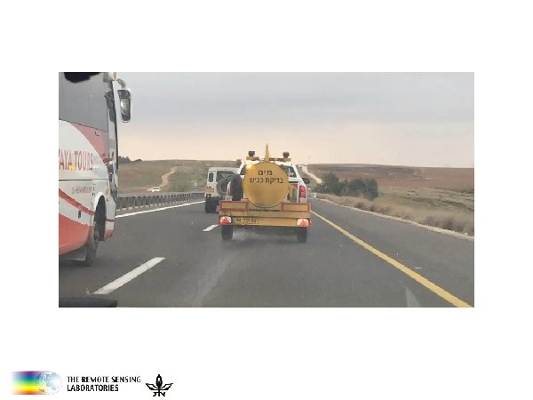
Dynamic Friction Mapping Today • • • The 5 th wheel concept Mechanical system Many disadvantages

VIS-NIR-SWIR region Ground • Spectrometer acquisition – Sensor: ASD – Research Area: 5 km segment of Road 4 – Flight height: 40 cm – Spectral sensitivity: VIS-NIR-SWIR – Spectral resolution: 2150 bands

Reflectance Wavelength (nm)

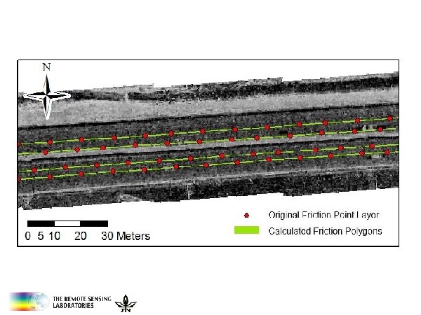
Data Processing Steps: 1. Pairing 2. Merging 3. Modeling ~10 m ~30 m

Machine Learning Spectral Information Chemical Attribute p. H COx Salt Clay Minerals We need a BIG dataset of samples for creating a VALID correlation model Then, we can predict the chemistry from the spectral data

Machine Learning Analysis PARACUDA II

Modeling

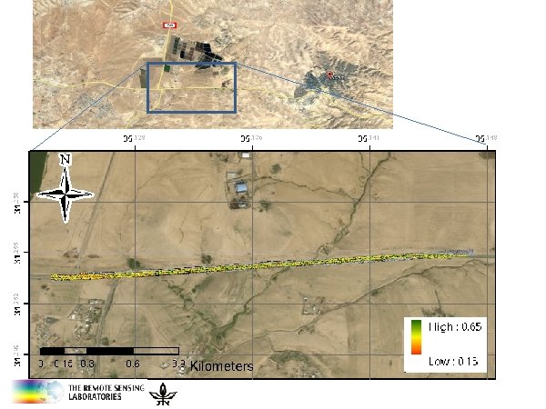
Airborne –VNIR-SWIR • Aerial acquisition campaign 380 -2500 nm 4. 5 -14 nm

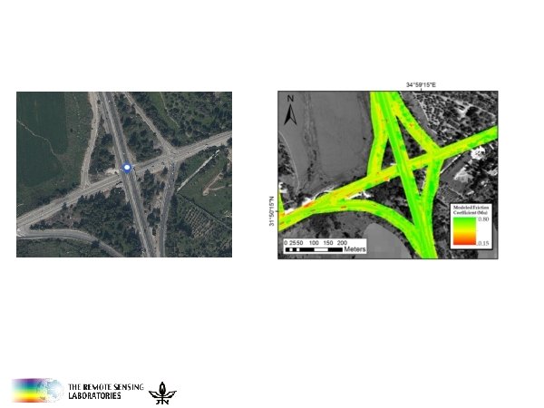
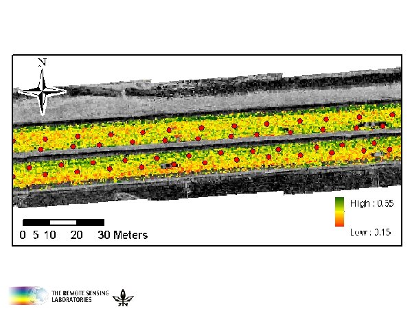
Working Scheme Data Acquisition over a selected high way “latron” Acquisition with the FENIX 1 K sensor Friction Coefficient by the “Israel ways” Geo rectification – FENIX 1 K Atmosphere Correction Data Mining Full spectrum (PLS + field Model)

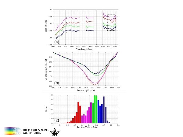
Calibration (b) validation ( c )

SWIR-1 B Coefficient VNIR Wavelength (nm) SWIR-2

Predicted (Mu) R 2 = 0. 6316 RMSEP = 0. 0776 RPD = 1. 6462 N= 1332 P<0. 0001 Measured (Mu) (a) R 2 = 0. 702 RMSEP = 0. 0696 RPD = 1. 8325 N= 333 P<0. 0001 Measured (Mu) (b)

TIR region Ground 25 20 F G Radiance 15 A 10 B C 5 0 D E 7. 5 8. 5 9. 5 10. 5 Wavelength (Microns)

Airborne –LWIR • Aerial acquisition campaign 7. 6 -11. 7 mm 4 cm-1; 70 bands www. telops. com

Airborne Operation 1. Collect airborne data of roads (RAD) 2. Obtain DFC data (Vehicle) 3. Correct spectral cubes for atmospheric attenuation and TES (FLASH IR) 4. Develop geometric tools for developing a dataset (TAU tool box) 5. Analyze dataset with data mining methods

Radiance TELOPS Geometric Correction FLASH IR TAU tool box Plank Fit Atmosphere Correction Emissivity Separation

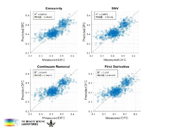
a Min Max Mean Std n 0. 22 0. 634 0. 45 0. 073 1055

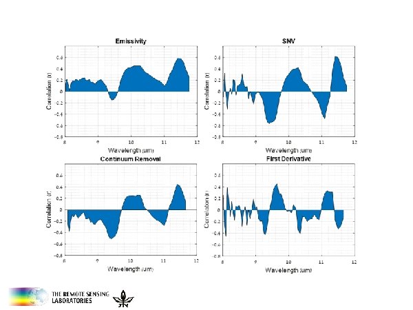
EMISIVITY AND FRICITION COEF

All Bands 88

11. 5 10. 3 11. 1 9. 4

4 Selected Bands 11. 5 11. 1 , 10. 3 , 9. 4

Road Margin Road Asphalt

The Vision HSR-TIR sensor Forward Looking TIR sensor

Conclusions 1. Airborne Hyperspectral Remote Sensing is capable to map the friction coefficient (FC) in asphaltic roads in both optical and thermal spectral regions 2. The VIS-NIR-SWIR is limited to day acquisition 3. The TIR is available is open for day and night acquisition 4. The FC can be extracted using only 4 channels only from the LWIR region. 5. Future vision: adopting the technology for safty driving and autonomous cars

Thank you for your attention!