Map Reduce Basics Algorithm Design By J H

Map. Reduce Basics & Algorithm Design By J. H. Wang May 9, 2017

Outline • Introduction • Map. Reduce Basics • Map. Reduce Algorithm Design

Reference • Jimmy Lin and Chris Dyer, “Data-Intensive Text Processing with Map. Reduce”, Ch. 1 -3 • Slides from Jimmy Lin’s “Big Data Infrastructure” course, Univ. Maryland (and Univ. Waterloo)

Divide and Conquer “Work” Partition w 1 w 2 w 3 worker r 1 r 2 r 3 “Result” Combine

Parallelization Challenges • How do we assign work units to workers? • What if we have more work units than workers? • What if workers need to share partial results? • How do we aggregate partial results? • How do we know all the workers have finished? • What if workers die? What'’s the common theme of all of these problems?

Common Theme? • Parallelization problems arise from: – Communication between workers (e. g. , to exchange state) – Access to shared resources (e. g. , data) • Thus, we need a synchronization mechanism

Managing Multiple Workers • Difficult because – – We don’t know the order in which workers run We don’t know when workers interrupt each other We don’t know when workers need to communicate partial results We don’t know the order in which workers access shared data • Thus, we need: – Semaphores (lock, unlock) – Conditional variables (wait, notify, broadcast) – Barriers • Still, lots of problems: – Deadlock, livelock, race conditions. . . – Dining philosophers, sleeping barbers, cigarette smokers. . . • Moral of the story: be careful!

Current Tools master Message Passing Shared Memory • Programming models – Shared memory (pthreads) – Message passing (MPI) • Design Patterns – Master-slaves – Producer-consumer flows – Shared work queues P 1 P 2 P 3 P 4 P 5 producer consumer work queue slaves producer consumer

Where the rubber meets the road • Concurrency is difficult to reason about • Concurrency is even more difficult to reason about – At the scale of datacenters and across datacenters – In the presence of failures – In terms of multiple interacting services • Not to mention debugging… • The reality: – Lots of one-off solutions, custom code – Write you own dedicated library, then program with it – Burden on the programmer to explicitly manage everything

Big Ideas behind Map. Reduce • Scale “out”, not “up” – A large number of commodity low-end servers is preferred over a small number of high-end servers • Assume failures are common – Fault-tolerant service must cope with failures without impacting the quality of service • Moving processing to the data – Map. Reduce assumes an architecture where processors and storage are co-located

• Processing data sequentially and avoid random access – Map. Reduce is primarily designed for batch processing over large datasets • Hide system-level details from the application developer – Simple and well-defined interfaces between a small number of components • Seamless scalability

Map. Reduce Basics

Map. Reduce Programming Model • Functional programming roots – Map and fold • • Mappers and reducers Execution framework Combiners and partitioners Distributed file system

Typical Big Data Problem Map • • • Iterate over a large number of records Extract something of interest from each ce results u d Shuffle and sort intermediate e R Aggregate intermediate results Generate final output Key idea: provide a functional abstraction for these two operations (Dean and Ghemawat, OSDI 2004)

Roots in Functional Programming Map f f f Fold g g g

Map. Reduce • Programmers specify two functions: map (k 1, v 1) → [<k 2, v 2>] reduce (k 2, [v 2]) → [<k 3, v 3>] – All values with the same key are sent to the same reducer • The execution framework handles everything else…

k 1 v 1 k 2 v 2 map a 1 k 3 v 3 k 4 v 4 map b 2 c 3 c k 5 v 5 k 6 v 6 map 6 a 5 c map 2 b 7 c Shuffle and Sort: aggregate values by keys a 1 5 b 2 7 c 2 3 6 8 reduce r 1 s 1 r 2 s 2 r 3 s 3 8

Map. Reduce • Programmers specify two functions: map (k, v) → <k’, v’>* reduce (k’, v’) → <k’, v’>* – All values with the same key are sent to the same reducer • The execution framework handles everything else… What’s “everything else”?

Map. Reduce “Runtime” • Handles scheduling – Assigns workers to map and reduce tasks • Handles “data distribution” – Moves processes to data • Handles synchronization – Gathers, sorts, and shuffles intermediate data • Handles errors and faults – Detects worker failures and restarts • Everything happens on top of a distributed FS

Map. Reduce • Programmers specify two functions: map (k, v) → <k’, v’>* reduce (k’, v’) → <k’, v’>* – All values with the same key are reduced together • The execution framework handles everything else… • Not quite…usually, programmers also specify: partition (k’, number of partitions) → partition for k’ – Often a simple hash of the key, e. g. , hash(k’) mod n – Divides up key space for parallel reduce operations combine (k’, v’) → <k’, v’>* – Mini-reducers that run in memory after the map phase – Used as an optimization to reduce network traffic

k 1 v 1 k 2 v 2 map a 1 k 4 v 4 map b 2 c combine a 1 k 3 v 3 3 c c partition k 6 v 6 map 6 a 5 combine b 2 k 5 v 5 c map 2 b 7 combine 9 a 5 partition c 1 5 2 b 7 partition b 2 7 8 combine c partition Shuffle and Sort: aggregate values by keys a c c 2 3 9 6 8 reduce r 1 s 1 r 2 s 2 r 3 s 3 8

Two more details… • Barrier between map and reduce phases – But we can begin copying intermediate data earlier • Keys arrive at each reducer in sorted order – No enforced ordering across reducers

“Hello World”: Word Count Map(String docid, String text): for each word w in text: Emit(w, 1); Reduce(String term, Iterator<Int> values): int sum = 0; for each v in values: sum += v; Emit(term, value);

Map. Reduce can refer to… • The programming model • The execution framework (aka “runtime”) • The specific implementation Usage is usually clear from context!

User Program (1) submit Master (2) schedule map (2) schedule reduce worker split 0 split 1 split 2 split 3 split 4 (5) remote read (3) read worker (4) local write worker (6) write output file 0 output file 1 worker Input files Adapted from (Dean and Ghemawat, OSDI 2004) Map phase Intermediate files (on local disk) Reduce phase Output files

Basic Hadoop API* • Mapper – void setup(Mapper. Context context) Called once at the beginning of the task – void map(K key, V value, Mapper. Context context) Called once for each key/value pair in the input split – void cleanup(Mapper. Context context) Called once at the end of the task • Reducer/Combiner – void setup(Reducer. Context context) Called once at the start of the task – void reduce(K key, Iterable<V> values, Reducer. Context context) Called once for each key – void cleanup(Reducer. Context context) Called once at the end of the task *Note that there are two versions of the A

Basic Hadoop API* • Partitioner – int get. Partition(K key, V value, int num. Partitions) Get the partition number given total number of partitions • Job – – – – Represents a packaged Hadoop job for submission to cluster Need to specify input and output paths Need to specify input and output formats Need to specify mapper, reducer, combiner, partitioner classes Need to specify intermediate/final key/value classes Need to specify number of reducers (but not mappers, why? ) Don’t depend of defaults! *Note that there are two versions of the A

“Hello World”: Word Count private static class My. Mapper extends Mapper<Long. Writable, Text, Int. Writable> { private final static Int. Writable ONE = new Int. Writable(1); private final static Text WORD = new Text(); @Override public void map(Long. Writable key, Text value, Context context) throws IOException, Interrupted. Exception { String line = ((Text) value). to. String(); String. Tokenizer itr = new String. Tokenizer(line); while (itr. has. More. Tokens()) { WORD. set(itr. next. Token()); context. write(WORD, ONE); } } }

“Hello World”: Word Count private static class My. Reducer extends Reducer<Text, Int. Writable, Text, Int. Writable> { private final static Int. Writable SUM = new Int. Writable(); @Override public void reduce(Text key, Iterable<Int. Writable> values, Context context) throws IOException, Interrupted. Exception { Iterator<Int. Writable> iter = values. iterator(); int sum = 0; while (iter. has. Next()) { sum += iter. next(). get(); } SUM. set(sum); context. write(key, SUM); } }

Word Count: the pseudo code

Input File Input. Split Record. Reader Mapper Mapper Input. Format Input. Split Intermediates Source: redrawn from a slide by Cloduera, cc-licensed Intermediates

Client Records … Input. Split Record. Reader Mapper

Mapper Mapper Intermediates Intermediates Partitioner Partitioner (combiners omitted here) Intermediates Reducer Source: redrawn from a slide by Cloduera, cc-licensed Intermediates Reducer Intermediates Reduce

Output. Format Reducer Reduce Record. Writer Output File Source: redrawn from a slide by Cloduera, cc-licensed

Shuffle and Sort in Hadoop • Probably the most complex aspect of Map. Reduce • Map side – Map outputs are buffered in memory in a circular buffer – When buffer reaches threshold, contents are “spilled” to disk – Spills merged in a single, partitioned file (sorted within each partition): combiner runs during the merges • Reduce side – First, map outputs are copied over to reducer machine – “Sort” is a multi-pass merge of map outputs (happens in memory and on disk): combiner runs during the merges – Final merge pass goes directly into reducer

Shuffle and Sort Mapper merged spills (on disk) intermediate files (on disk) Combiner circular buffer (in memory) Combiner spills (on disk) other mappers other reducers Reducer

Hadoop Workflow 1. Load data into HDFS 2. Develop code locally 3. Submit Map. Reduce job 3 a. Go back to Step 2 You Hadoop Cluster 4. Retrieve data from HDFS

Recommended Workflow • Here’s how I work: – – – – – Develop code in Eclipse on host machine Build distribution on host machine Check out copy of code on VM Copy (i. e. , scp) jars over to VM (in same directory structure) Run job on VM Iterate … Commit code on host machine and push Pull from inside VM, verify • Avoid using the UI of the VM – Directly ssh into the VM

Debugging Hadoop • First, take a deep breath • Start small, start locally • Build incrementally

Code Execution Environments • Different ways to run code: – Plain Java – Local (standalone) mode – Pseudo-distributed mode – Fully-distributed mode • Learn what’s good for what

Hadoop Debugging Strategies • Good ol’ System. out. println – Learn to use the webapp to access logs – Logging preferred over System. out. println – Be careful how much you log! • Fail on success – Throw Runtime. Exceptions and capture state • Programming is still programming – Use Hadoop as the “glue” – Implement core functionality outside mappers and reducers – Independently test (e. g. , unit testing) – Compose (tested) components in mappers and reducers

Example: Word. Count in Action • Environment variables setting: – export JAVA_HOME=/usr/java/default – export PATH=${JAVA_HOME}/bin: ${PATH} – export HADOOP_CLASSPATH=${JAVA_HOME}/lib/tools. jar • Compiling java code to create a jar: – cd ${HADOOP_HOME}/src/examples – ${HADOOP_HOME}/bin/hadoop com. sun. tools. javac. Main org/apache/hadoop/examples/Word. Count. java – jar cf wc. jar org/apache/hadoop/examples/Word. Count*. class • Running the application in jar: – ${HADOOP_HOME}/bin/hadoop jar wc. jar org. apache. hadoop. examples. Word. Count <in> <out> – * NOTE: <in> and <out> are directories in HDFS

Map. Reduce Algorithm Design

Major Issues in Map. Reduce Algorithm Design • Synchronization – The most tricky aspect of designing Map. Reduce algorithms – The only cluster-wide synchronization during shuffle and sort stage: from mapper to reducer • Techniques to control execution and data flow in Map. Reduce – Scalability – Efficiency

• Limited control over data and execution flow – Where mappers and reducers run – When a mapper or reducer begins or finishes – Which input a particular mapper is processing – Which intermediate key a particular reducer is processing

Tools for Synchronization • Cleverly-constructed data structures – Bring partial results together • Sort order of intermediate keys – Control order in which reducers process keys • Partitioner – Control which reducer processes which keys • Preserving state in mappers and reducers – Capture dependencies across multiple keys and values

Preserving State Mapper object state setup map Reducer object one object per task API initialization hook one call per input key-value pair state setup reduce one call per intermediate key cleanup API cleanup hook close

Scalable Hadoop Algorithms: Themes • Avoid object creation – Inherently costly operation – Garbage collection • Avoid buffering – Limited heap size – Works for small datasets, but won’t scale!

Importance of Local Aggregation • Ideal scaling characteristics: – Twice the data, twice the running time – Twice the resources, half the running time • Why can’t we achieve this? – Synchronization requires communication – Communication kills performance • Thus… avoid communication! – Reduce intermediate data via local aggregation – Combiners can help

Local Aggregation • The single most important aspect of synchronization in data-intensive distributed processing – The exchange of intermediate results • Intermediate results: mapper -> reducer • written to disk, and sent over the network • Expensive – Local aggregation of intermediate results • Using the combiner • To preserve state across multiple inputs

Shuffle and Sort Mapper merged spills (on disk) intermediate files (on disk) Combiner circular buffer (in memory) Combiner spills (on disk) other mappers other reducers Reducer

Word Count: Baseline What’s the impact of combiners?

Word Count: Version 1 Are combiners still needed?

Word Count: Version 2 te a t s e v er irs! s e r a p p : a e e u l d i a v Key t keyu inp Are combiners still needed? ss o r ac

The “in-mapper combining” Design Pattern • Combiners: to reduce the amount of intermediate results generated by mappers – Mini-reducers: mapper -> combiner -> reducer • In-mapper combining – Provide control over when local aggregation occurs and how it exactly takes place • Advantages – Speed – Why is this faster than actual combiners? • Disadvantages – Explicit memory management required – Potential for order-dependent bugs

• Drawbacks of in-mapper combining – Breaks the functional programming underpinnings of Map. Reduce • Preserving state across multiple input instances means that algorithmic behavior may depend on the order of input key-value pairs – Fundamental scalability bottleneck • Memory usage in the mapper – The associative array might not fit in memory

• Solution – Limiting the memory usage when using the inmapper combining technique • To block input key-value pairs • To flush in-memory data structures periodically • Emitting intermediate results every n key-value pairs – Counter – Threshold on memory usage

• Factors affecting the efficiency improvement with local aggregation – Size of the intermediate key space – Distribution of keys – Number of key-value pairs that are emitted by each map task • Opportunities from aggregation come from having multiple values associated with the same key • Effective for reduce stragglers that result from a highly skewed distribution of values

Algorithm correctness with local aggregation • Reducer input key-value type must match mapper output key-value type – Combiner input and output key-value types must match mapper output key-value type – Mapper -> combiner -> reducer • In general, combiners and reducers are not interchangeable – Reducers can be used as combiners when the reduce operation is both commutative and associative

Combiner Design • Combiners and reducers share same method signature – Sometimes, reducers can serve as combiners – Often, not… • Remember: combiner are optional optimizations – Should not affect algorithm correctness – May be run 0, 1, or multiple times • Example: find average of integers associated with the same key

Computing the Mean: Version 1 Why can’t we use reducer as combiner?

Computing the Mean: Version 2 Why doesn’t this work?

Computing the Mean: Version 3 Fixed?

Computing the Mean: Version 4 Are combiners still needed?

Pairs and Stripes • References: – Chris Dyer, Aaron Cordova, Alex Mont, and Jimmy Lin, “Fast, easy, and cheap: Construction of statistical machine translation models with Map. Reduce, ” Proceedings of the 3 rd workshop on Statistical Machine Translation at ACL 2008, pp. 199 -207, 2008. – Jimmy Lin, “Scalable language processing algorithms for the masses: A case study in computing word cooccurrence matrices with Map. Reduce, ” Proceedings of the 2008 Conference on Empirical Methods in Natural Language Processing (EMNLP 2008), pp. 419428, 2008.

Algorithm Design: Running Example • Term co-occurrence matrix for a text collection – M = N x N matrix (N = vocabulary size) – Mij: number of times wi and wj co-occur in some context (for concreteness, let’s say context = sentence) • Why? – Distributional profiles as a way of measuring semantic distance – Semantic distance useful for many language processing tasks

Map. Reduce: Large Counting Problems • Term co-occurrence matrix for a text collection = specific instance of a large counting problem – A large event space (number of terms) – A large number of observations (the collection itself) – Goal: keep track of interesting statistics about the events • Basic approach – Mappers generate partial counts – Reducers aggregate partial counts How do we aggregate partial counts efficiently?

First Try: “Pairs” • The use of complex keys to coordinate distributed computations • Each mapper takes a sentence: – Generate all co-occurring term pairs – For all pairs, emit (a, b) → count • Reducers sum up counts associated with these pairs • Use combiners!

Pairs: Pseudo-Code

“Pairs” Analysis • Advantages – Easy to implement, easy to understand • Disadvantages – Lots of pairs to sort and shuffle around (upper bound? ) – Not many opportunities for combiners to work

Another Try: “Stripes” • Idea: group together pairs into an associative array (a, b) → 1 (a, c) → 2 (a, d) → 5 (a, e) → 3 (a, f) → 2 a → { b: 1, c: 2, d: 5, e: 3, f: 2 } • Each mapper takes a sentence: – Generate all co-occurring term pairs – For each term, emit a → { b: countb, c: countc, d: countd … } re uctu tr s a t • Reducers perform element-wise sum of associative d da e t c + tru s arrays n o ults ly-c a → { b: 1, d: 5, e: 3 } res ver l e l a i c t ar a → { b: 1, c: 2, d: 2, f: 2 } idea: p r e y th e a → { b: 2, c: 2, d: 7, e: 3, f: K 2 } gs toge brin

Stripes: Pseudo-Code

“Stripes” Analysis • Advantages – Far less sorting and shuffling of key-value pairs – Can make better use of combiners • Disadvantages – More difficult to implement – Underlying object more heavyweight – Fundamental limitation in terms of size of event space

Comparisons • Pairs: – Huge number of key-value pairs • Stripes: – More compact representation – Fewer intermediate keys, less sorting – More complex values, more serialization and deserialization overhead

• Both can benefit from the use of combiners – But, stripes approach can have more opportunities to perform local aggregation since the key space is the vocabulary • In-mapper combining optimization can both be applied – But, far fewer opportunities for partial aggregation in the pairs approach due to the sparsity of the intermediate key space • Memory management will be more complex for the stripes approach – Assumption: each associative array is small enough to fit into memory

A Brief Summary • Pairs – Individually records each co-occurring event • Stripes – Records all co-occurring events with respect to a conditioning event

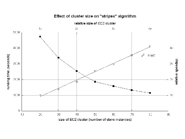
Cluster size: 38 cores Data Source: Associated Press Worldstream (APW) of the English Gigaword Corpus (v 3), which contains 2. 27 million documents (1. 8 GB compressed, 5. 7 GB uncompressed)

Computing Relative Frequencies • To convert absolute counts into relative frequencies f(wj|wi) – Straightforward in the stripes approach • Pairs: – We have to properly sequence data presented to the reducer • The programmer can define the sort order of keys so that data needed earlier is presented to the reducer before other data • In the reducer, we have to define the sort order of the keys so that pairs with special symbol (wi, *) are ordered before any other key-value pairs with wi

Relative Frequencies • How do we estimate relative frequencies from counts? • Why do we want to do this? • How do we do this with Map. Reduce?

f(B|A): “Stripes” a → {b 1: 3, b 2 : 12, b 3 : 7, b 4 : 1, … } • Easy! – One pass to compute (a, *) – Another pass to directly compute f(B|A)

f(B|A): “Pairs” • What’s the issue? – Computing relative frequencies requires marginal counts – But the marginal cannot be computed until you see all counts – Buffering is a bad idea! • Solution: – What if we could get the marginal count to arrive at the reducer first?

f(B|A): “Pairs” (a, *) → 32 Reducer holds this value in memory (a, b 1) → 3 (a, b 2) → 12 (a, b 3) → 7 (a, b 4) → 1 … • For this to work: (a, b 1) → 3 / 32 (a, b 2) → 12 / 32 (a, b 3) → 7 / 32 (a, b 4) → 1 / 32 … – Must emit extra (a, *) for every bn in mapper – Must make sure all a’s get sent to same reducer (use partitioner) – Must make sure (a, *) comes first (define sort order) – Must hold state in reducer across different key-value pairs

“Order Inversion” • Common design pattern: – Take advantage of sorted key order at reducer to sequence computations – Get the marginal counts to arrive at the reducer before the joint counts • Optimization: – Apply in-memory combining pattern to accumulate marginal counts

Synchronization: Pairs vs. Stripes • Approach 1: turn synchronization into an ordering problem – Sort keys into correct order of computation – Partition key space so that each reducer gets the appropriate set of partial results – Hold state in reducer across multiple key-value pairs to perform computation – Illustrated by the “pairs” approach • Approach 2: construct data structures that bring partial results together – Each reducer receives all the data it needs to complete the computation – Illustrated by the “stripes” approach

Order inversion • Through proper coordination, we can access the result of a computation in the reducer before processing the data needed for that computation – To convert the sequencing of computations into a sorting problem

A brief summary • Requirements of order inversion: – Emitting a special key-value pair for each co-occurring word pair in the mapper – Controlling the sort order of the intermediate key so that the key-value pairs representing the marginal contributions are processed by the reducer before any other pairs – Defining a custom partitioner to ensure that all pairs with the same left word are shuffled to the same reducer – Preserving state across multiple keys in the reducer

Secondary Sorting • Map. Reduce sorts input to reducers by key – Values may be arbitrarily ordered • What if we want to sort by value also? – E. g. , k → (v 1, r), (v 3, r), (v 4, r), (v 8, r)…

Secondary Sorting: Solutions • Solution 1: – Buffer values in memory, then sort – Why is this a bad idea? • Solution 2: – “Value-to-key conversion” design pattern: form composite intermediate key, (k, v 1) – Let execution framework do the sorting – Preserve state across multiple key-value pairs to handle processing – Anything else we need to do?

Secondary Sorting • What if we need to sort by value in addition to sorting by key? – Google’s Map. Reduce provides built-in functionality for this, but Hadoop doesn’t • We need “value-to-key conversion” – To move part of the value into the intermediate key to form a composite key, and let Map. Reduce execution framework handle the sorting

• Basic tradeoff between buffer and in-memory sort vs. value-to-key conversion – Where sorting is performed • In Reducer: scalability bottleneck • In Map. Reduce execution framework: distributed sorting

Value-to-Key Conversion Before k → (v 1, r), (v 4, r), (v 8, r), (v 3, r)… Values arrive in arbitrary order… After (k, v 1) → (v 1, r) (k, v 3) → (v 3, r) (k, v 4) → (v 4, r) (k, v 8) → (v 8, r) … Values arrive in sorted order… Process by preserving state across multiple keys Remember to partition correctly!

Working Scenario • Two tables: – User demographics (gender, age, income, etc. ) – User page visits (URL, time spent, etc. ) • Analyses we might want to perform: – Statistics on demographic characteristics – Statistics on page visits by URL – Statistics on page visits by demographic characteristic –…

Relational Algebra • Primitives – Projection ( ) – Selection ( ) – Cartesian product ( ) – Set union ( ) – Set difference ( ) – Rename ( ) • Other operations – Join (⋈) – Group by… aggregation –…

Projection R 1 R 2 R 3 R 4 R 5

Projection in Map. Reduce • Easy! – Map over tuples, emit new tuples with appropriate attributes – No reducers, unless for regrouping or resorting tuples – Alternatively: perform in reducer, after some other processing • Basically limited by HDFS streaming speeds – Speed of encoding/decoding tuples becomes important – Take advantage of compression when available – Semistructured data? No problem!

Selection R 1 R 2 R 3 R 4 R 5 R 1 R 3

Selection in Map. Reduce • Easy! – Map over tuples, emit only tuples that meet criteria – No reducers, unless for regrouping or resorting tuples – Alternatively: perform in reducer, after some other processing • Basically limited by HDFS streaming speeds – Speed of encoding/decoding tuples becomes important – Take advantage of compression when available – Semistructured data? No problem!

Group by… Aggregation • Example: What is the average time spent per URL? • In SQL: – SELECT url, AVG(time) FROM visits GROUP BY url • In Map. Reduce: – Map over tuples, emit time, keyed by url – Framework automatically groups values by keys – Compute average in reducer – Optimize with combiners

Relational Joins R 1 S 1 R 2 S 2 R 3 S 3 R 4 S 4 R 1 S 2 R 2 S 4 R 3 S 1 R 4 S 3

Types of Relationships

Relational Joins • Reduce-side Join • Map-side Join • Memory-backed Join – Striped variant – Memcached variant

Reduce-Side Join • Reduce-Side Join – “parallel sort-merge join”: Map over both datasets, emit the join key as the intermediate key, and the tuple itself as the intermediate value – 3 cases: • One-to-one • one-to-many: scalability, secondary sort needed • many-to-many – Basic idea: to repartition the two datasets by the join key • Not efficient: shuffling both datasets across the network

Reduce-side Join • Basic idea: group by join key – Map over both sets of tuples – Emit tuple as value with join key as the intermediate key – Execution framework brings together tuples sharing the same key – Perform actual join in reducer – Similar to a “sort-merge join” in database terminology • Two variants – 1 -to-1 joins – 1 -to-many and many-to-many joins

Reduce-side Join: 1 -to-1 Map keys values R 1 R 4 S 2 S 3 Reduce keys values R 1 S 2 S 3 R 4 Note: no guarantee if R is going to come first or S

Map Reduce-side Join: 1 -to-many keys values R 1 S 2 S 3 S 9 Reduce keys values R 1 S 2 What’s S 3 ? m e l b o the pr …

Reduce-side Join: V-to-K Conversion In reducer… keys values R 1 New key encountered: hold in memory S 2 Cross with records from other set S 3 S 9 R 4 New key encountered: hold in memory S 3 Cross with records from other set S 7

Reduce-side Join: many-to-many In reducer… keys values R 1 R 5 Hold in memory R 8 Cross with records from other set S 2 S 3 S 9 What’s ? m e l b o the pr

Map-side Join: Basic Idea Assume two datasets are sorted by the join key: R 1 S 2 R 2 S 4 R 4 S 3 R 3 S 1 A sequential scan through both datasets to join (called a “merge join” in database terminology)

Map-Side Join • Map-side Join – Scanning through both datasets simultaneously (merge join) in the mapper • Both partitioned and sorted in the same manner by the join key • Map over the larger dataset, and inside the mapper read the corresponding part of the other dataset to perform the merge join – Far more efficient than reduce-side join – Restriction: it depends on consistent partitioning and sorting of keys

Map-side Join: Parallel Scans • If datasets are sorted by join key, join can be accomplished by a scan over both datasets • How can we accomplish this in parallel? – Partition and sort both datasets in the same manner • In Map. Reduce: – Map over one dataset, read from other corresponding partition – No reducers necessary (unless to repartition or resort) • Consistently partitioned datasets: realistic to expect?

In-Memory Join • Basic idea: load one dataset into memory, stream over other dataset – Works if R << S and R fits into memory – Called a “hash join” in database terminology • Map. Reduce implementation – Distribute R to all nodes – Map over S, each mapper loads R in memory, hashed by join key – For every tuple in S, look up join key in R – No reducers, unless for regrouping or resorting tuples

In-Memory Join: Variants • Striped variant: – R too big to fit into memory? – Divide R into R 1, R 2, R 3, … s. t. each Rn fits into memory – Perform in-memory join: n, Rn ⋈ S – Take the union of all join results • Memcached join: – Load R into memcached, a distributed key-value store – Replace in-memory hash lookup with memcached lookup

Memcached Circa 2008 Architecture Caching servers: 15 million requests per second, 95% handled by memcache (15 TB of RAM) Database layer: 800 eight-core Linux servers running My. SQL (40 TB user data) Source: Technology Review (July/August, 2008)

Memcached Join • Memcached join: – Load R into memcached – Replace in-memory hash lookup with memcached lookup • Capacity and scalability? – Memcached capacity >> RAM of individual node – Memcached scales out with cluster • Latency? – Memcached is fast (basically, speed of network) – Batch requests to amortize latency costs Source: See tech report by Lin et al. (2009)

Which join to use? • In-memory join > map-side join > reduce-side join – Why? • Limitations of each? – In-memory join: memory – Map-side join: sort order and partitioning – Reduce-side join: general purpose

Processing Relational Data: Summary • Map. Reduce algorithms for processing relational data: – Group by, sorting, partitioning are handled automatically by shuffle/sort in Map. Reduce – Selection, projection, and other computations (e. g. , aggregation), are performed either in mapper or reducer – Multiple strategies for relational joins • Complex operations require multiple Map. Reduce jobs – Example: top ten URLs in terms of average time spent – Opportunities for automatic optimization

Summary • Design patterns: – In-mapper combining: local aggregation – Pairs and stripes – Order inversion – Value-to-key conversion: secondary sort

Limitations of Map. Reduce • Many examples of algorithms depend crucially on the existence of shared global state during processing -> difficult to implement in Map. Reduce – Online learning • The model parameters in a learning algorithm can be viewed as shared global state – The framework must be altered to support faster processing of smaller datasets • Map. Reduce was specially optimized for “batch” operations over large amounts of data – Monte Carlo simulations

• Possible solution: distributed datastore capable of maintaining global state – Google’s Big. Table (or Hbase) – Amazon’s Dynamo (or Cassandra) • Alternative computing paradigms – Dryad: arbitrary dataflow graphs – Pregel: large-scale graph processing • BSP model

Thanks for Your Attention!