Manifold Clustering with Applications to Computer Vision and

Manifold Clustering with Applications to Computer Vision and Diffusion Imaging René Vidal Center for Imaging Science Institute for Computational Medicine Johns Hopkins University

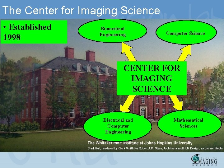
The Center for Imaging Science • Established 1998 Biomedical Engineering Computer Science CENTER FOR IMAGING SCIENCE Electrical and Computer Engineering Mathematical Sciences

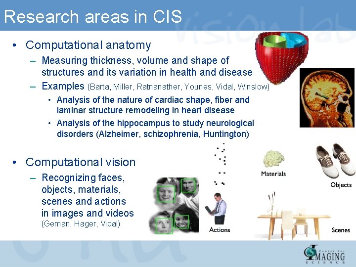
Research areas in CIS • Computational anatomy – Measuring thickness, volume and shape of structures and its variation in health and disease – Examples (Barta, Miller, Ratnanather, Younes, Vidal, Winslow) • Analysis of the nature of cardiac shape, fiber and laminar structure remodeling in heart disease • Analysis of the hippocampus to study neurological disorders (Alzheimer, schizophrenia, Huntington) • Computational vision – Recognizing faces, objects, materials, scenes and actions in images and videos (Geman, Hager, Vidal)

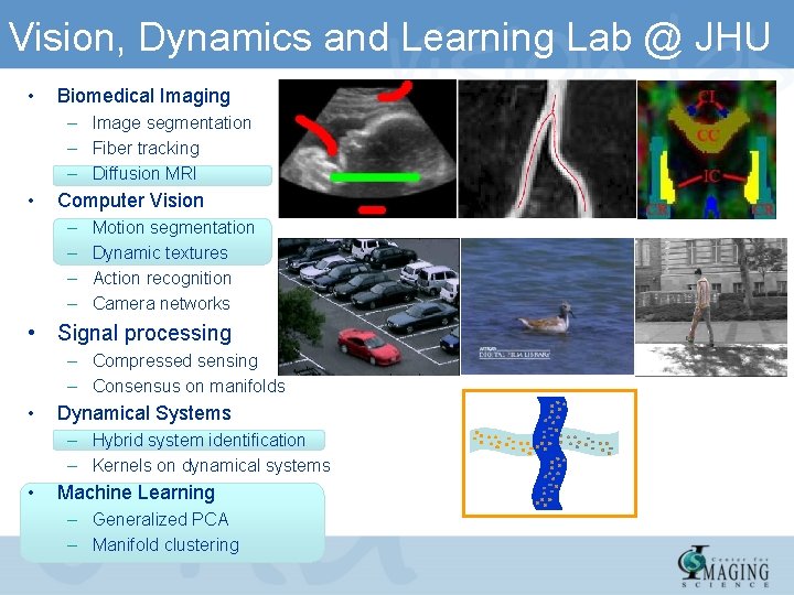
Vision, Dynamics and Learning Lab @ JHU • Biomedical Imaging – Image segmentation – Fiber tracking – Diffusion MRI • Computer Vision – – Motion segmentation Dynamic textures Action recognition Camera networks • Signal processing – Compressed sensing – Consensus on manifolds • Dynamical Systems – Hybrid system identification – Kernels on dynamical systems • Machine Learning – Generalized PCA – Manifold clustering

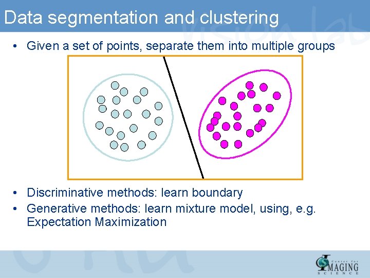
Data segmentation and clustering • Given a set of points, separate them into multiple groups • Discriminative methods: learn boundary • Generative methods: learn mixture model, using, e. g. Expectation Maximization

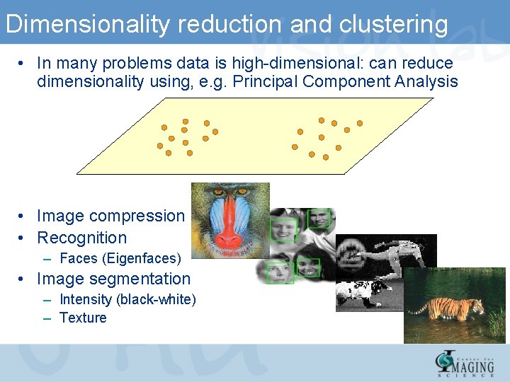
Dimensionality reduction and clustering • In many problems data is high-dimensional: can reduce dimensionality using, e. g. Principal Component Analysis • Image compression • Recognition – Faces (Eigenfaces) • Image segmentation – Intensity (black-white) – Texture

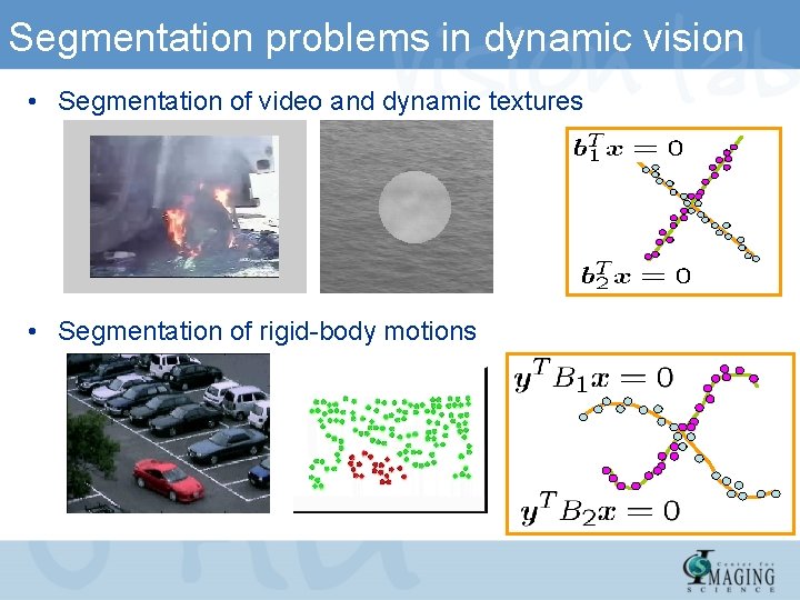
Segmentation problems in dynamic vision • Segmentation of video and dynamic textures • Segmentation of rigid-body motions

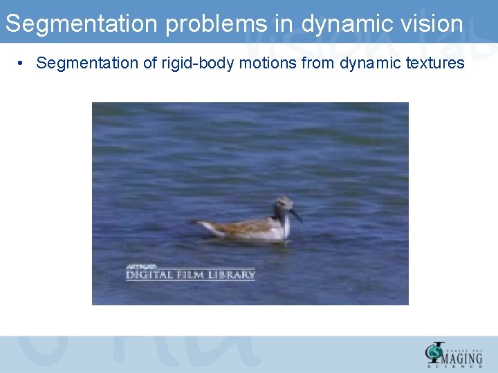
Segmentation problems in dynamic vision • Segmentation of rigid-body motions from dynamic textures

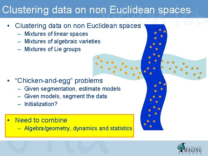
Clustering data on non Euclidean spaces • Clustering data on non Euclidean spaces – Mixtures of linear spaces – Mixtures of algebraic varieties – Mixtures of Lie groups • “Chicken-and-egg” problems – Given segmentation, estimate models – Given models, segment the data – Initialization? • Need to combine – Algebra/geometry, dynamics and statistics

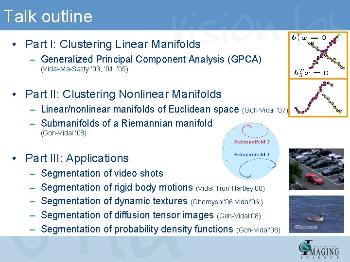
Talk outline • Part I: Clustering Linear Manifolds – Generalized Principal Component Analysis (GPCA) (Vidal-Ma-Sasty ’ 03, ‘ 04, ‘ 05) • Part II: Clustering Nonlinear Manifolds – Linear/nonlinear manifolds of Euclidean space (Goh-Vidal ‘ 07) – Submanifolds of a Riemannian manifold (Goh-Vidal ‘ 08) • Part III: Applications – – – Segmentation of video shots Segmentation of rigid body motions (Vidal-Tron-Hartley’ 08) Segmentation of dynamic textures (Ghoreyshi’ 06, Vidal’ 06 ) Segmentation of diffusion tensor images (Goh-Vidal’ 08) Segmentation of probability density functions (Goh-Vidal’ 08)

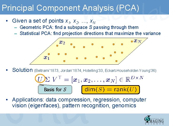
Principal Component Analysis (PCA) • Given a set of points x 1, x 2, …, x. N – Geometric PCA: find a subspace S passing through them – Statistical PCA: find projection directions that maximize the variance • Solution (Beltrami’ 1873, Jordan’ 1874, Hotelling’ 33, Eckart-Householder-Young’ 36) Basis for S • Applications: data compression, regression, computer vision (eigenfaces), pattern recognition, genomics

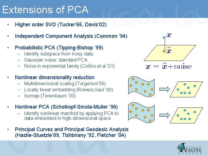
Extensions of PCA • Higher order SVD (Tucker’ 66, Davis’ 02) • Independent Component Analysis (Common ‘ 94) • Probabilistic PCA (Tipping-Bishop ’ 99) – Identify subspace from noisy data – Gaussian noise: standard PCA – Noise in exponential family (Collins et al. ’ 01) • Nonlinear dimensionality reduction – Multidimensional scaling (Torgerson’ 58) – Locally linear embedding (Roweis-Saul ’ 00) – Isomap (Tenenbaum ’ 00) • Nonlinear PCA (Scholkopf-Smola-Muller ’ 98) – Identify nonlinear manifold by applying PCA to data embedded in high-dimensional space • Principal Curves and Principal Geodesic Analysis (Hastie-Stuetzle’ 89, Tishbirany ‘ 92, Fletcher ‘ 04)

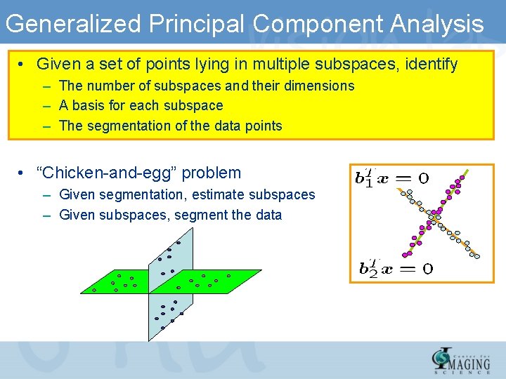
Generalized Principal Component Analysis • Given a set of points lying in multiple subspaces, identify – The number of subspaces and their dimensions – A basis for each subspace – The segmentation of the data points • “Chicken-and-egg” problem – Given segmentation, estimate subspaces – Given subspaces, segment the data

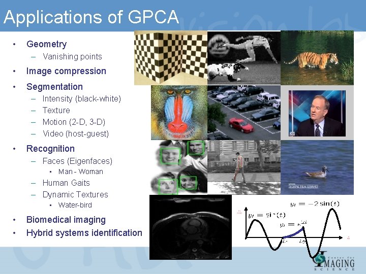
Applications of GPCA • Geometry – Vanishing points • Image compression • Segmentation – – • Intensity (black-white) Texture Motion (2 -D, 3 -D) Video (host-guest) Recognition – Faces (Eigenfaces) • Man - Woman – Human Gaits – Dynamic Textures • Water-bird • • Biomedical imaging Hybrid systems identification

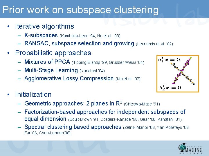
Prior work on subspace clustering • Iterative algorithms – K-subspaces (Kamhalta-Leen ‘ 94, Ho et al. ’ 03) – RANSAC, subspace selection and growing (Leonardis et al. ’ 02) • Probabilistic approaches – Mixtures of PPCA (Tipping-Bishop ’ 99, Grubber-Weiss ’ 04) – Multi-Stage Learning (Kanatani ’ 04) – Agglomerative Lossy Compression (Ma et al. ’ 07) • Initialization – Geometric approaches: 2 planes in R 3 (Shizawa-Maze ’ 91) – Factorization-based approaches for independent subspaces of equal dimension (Boult-Brown ‘ 91, Costeira-Kanade ‘ 98, Gear ’ 08, Kanatani ’ 01) – Spectral clustering based approaches (Zelnik-Manor ‘ 03, Yan-Pollefeys ’ 06, Fan’ 06, Chen-Lerman’ 08)

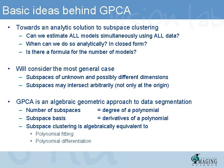
Basic ideas behind GPCA • Towards an analytic solution to subspace clustering – Can we estimate ALL models simultaneously using ALL data? – When can we do so analytically? In closed form? – Is there a formula for the number of models? • Will consider the most general case – Subspaces of unknown and possibly different dimensions – Subspaces may intersect arbitrarily (not only at the origin) • GPCA is an algebraic geometric approach to data segmentation – Number of subspaces = degree of a polynomial – Subspace basis = derivatives of a polynomial – Subspace clustering is algebraically equivalent to • Polynomial fitting • Polynomial differentiation

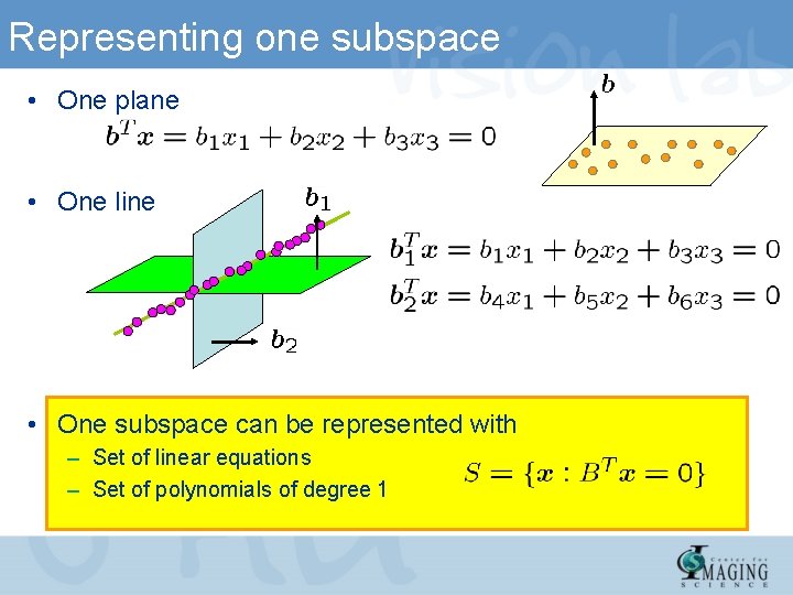
Representing one subspace • One plane • One line • One subspace can be represented with – Set of linear equations – Set of polynomials of degree 1

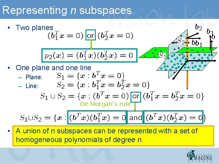
Representing n subspaces • Two planes • One plane and one line – Plane: – Line: De Morgan’s rule • A union of n subspaces can be represented with a set of homogeneous polynomials of degree n

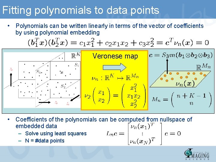
Fitting polynomials to data points • Polynomials can be written linearly in terms of the vector of coefficients by using polynomial embedding Veronese map • Coefficients of the polynomials can be computed from nullspace of embedded data – Solve using least squares – N = #data points

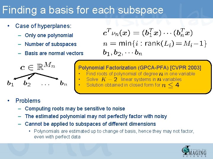
Finding a basis for each subspace • Case of hyperplanes: – Only one polynomial – Number of subspaces – Basis are normal vectors Polynomial Factorization (GPCA-PFA) [CVPR 2003] • • • Find roots of polynomial of degree in one variable Solve linear systems in variables Solution obtained in closed form for • Problems – Computing roots may be sensitive to noise – The estimated polynomial may not perfectly factor with noisy – Cannot be applied to subspaces of different dimensions • Polynomials are estimated up to change of basis, hence they may not factor, even with perfect data

Finding a basis for each subspace Polynomial Differentiation (GPCA-PDA) [CVPR’ 04] • To learn a mixture of subspaces we just need one positive example per class

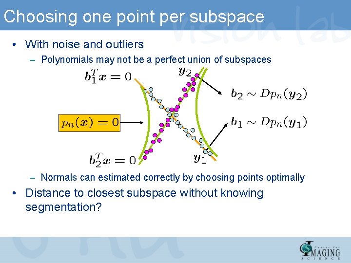
Choosing one point per subspace • With noise and outliers – Polynomials may not be a perfect union of subspaces – Normals can estimated correctly by choosing points optimally • Distance to closest subspace without knowing segmentation?

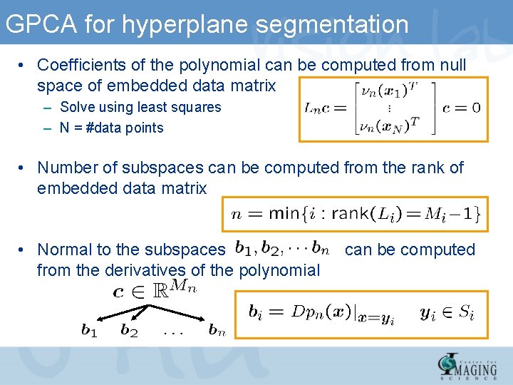
GPCA for hyperplane segmentation • Coefficients of the polynomial can be computed from null space of embedded data matrix – Solve using least squares – N = #data points • Number of subspaces can be computed from the rank of embedded data matrix • Normal to the subspaces from the derivatives of the polynomial can be computed

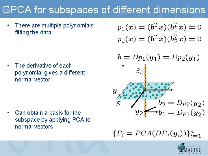
GPCA for subspaces of different dimensions • There are multiple polynomials fitting the data • The derivative of each polynomial gives a different normal vector • Can obtain a basis for the subspace by applying PCA to normal vectors

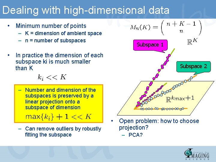
Dealing with high-dimensional data • Minimum number of points – K = dimension of ambient space – n = number of subspaces Subspace 1 • In practice the dimension of each subspace ki is much smaller than K Subspace 2 – Number and dimension of the subspaces is preserved by a linear projection onto a subspace of dimension – Can remove outliers by robustly fitting the subspace • Open problem: how to choose projection? – PCA?

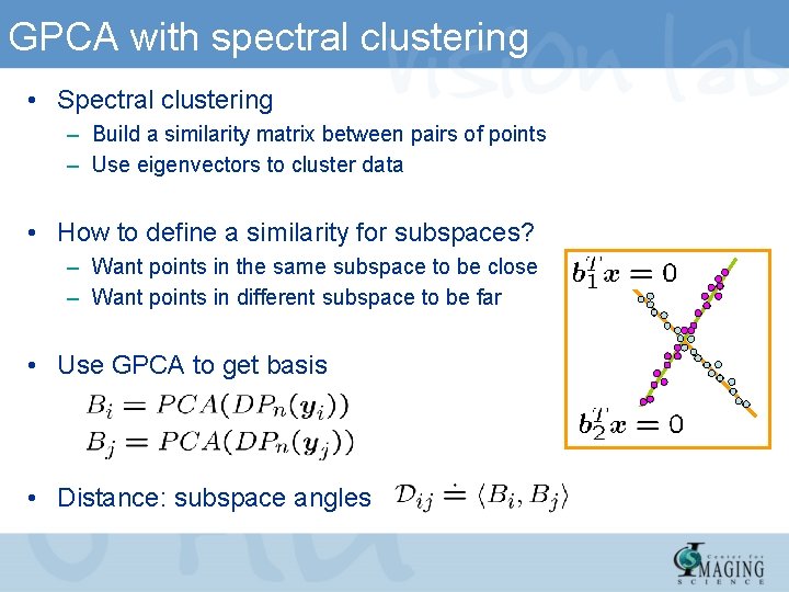
GPCA with spectral clustering • Spectral clustering – Build a similarity matrix between pairs of points – Use eigenvectors to cluster data • How to define a similarity for subspaces? – Want points in the same subspace to be close – Want points in different subspace to be far • Use GPCA to get basis • Distance: subspace angles

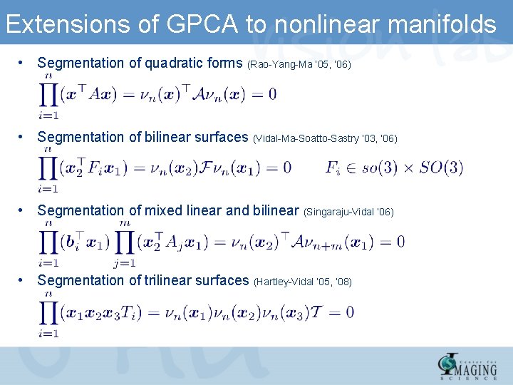
Extensions of GPCA to nonlinear manifolds • Segmentation of quadratic forms (Rao-Yang-Ma ’ 05, ‘ 06) • Segmentation of bilinear surfaces (Vidal-Ma-Soatto-Sastry ’ 03, ‘ 06) • Segmentation of mixed linear and bilinear (Singaraju-Vidal ‘ 06) • Segmentation of trilinear surfaces (Hartley-Vidal ’ 05, ’ 08)

Part II: Nonlinear Manifold Clustering René Vidal Center for Imaging Science Institute for Computational Medicine Johns Hopkins University

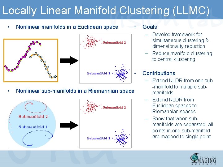
Locally Linear Manifold Clustering (LLMC) • Nonlinear manifolds in a Euclidean space • Goals – Develop framework for simultaneous clustering & dimensionality reduction – Reduce manifold clustering to central clustering • • Nonlinear sub-manifolds in a Riemannian space Contributions – Extend NLDR from one sub -manifold to multiple submanifolds – Extend NLDR from Euclidean spaces to Riemannian spaces – Show that when submanifolds are separated, all points in one sub-manifold are mapped to single point

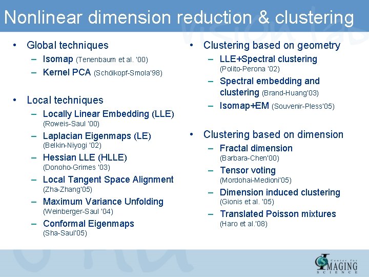
Nonlinear dimension reduction & clustering • Global techniques – Isomap (Tenenbaum et al. ‘ 00) – Kernel PCA (Schölkopf-Smola’ 98) • Local techniques – Locally Linear Embedding (LLE) • Clustering based on geometry – LLE+Spectral clustering (Polito-Perona ’ 02) – Spectral embedding and clustering (Brand-Huang’ 03) – Isomap+EM (Souvenir-Pless’ 05) (Roweis-Saul ’ 00) – Laplacian Eigenmaps (LE) (Belkin-Niyogi ‘ 02) – Hessian LLE (HLLE) (Donoho-Grimes ‘ 03) – Local Tangent Space Alignment (Zha-Zhang’ 05) – Maximum Variance Unfolding (Weinberger-Saul ‘ 04) – Conformal Eigenmaps (Sha-Saul’ 05) • Clustering based on dimension – Fractal dimension (Barbara-Chen’ 00) – Tensor voting (Mordohai-Medioni’ 05) – Dimension induced clustering (Gionis et al. ’ 05) – Translated Poisson mixtures (Haro et al. ’ 08)

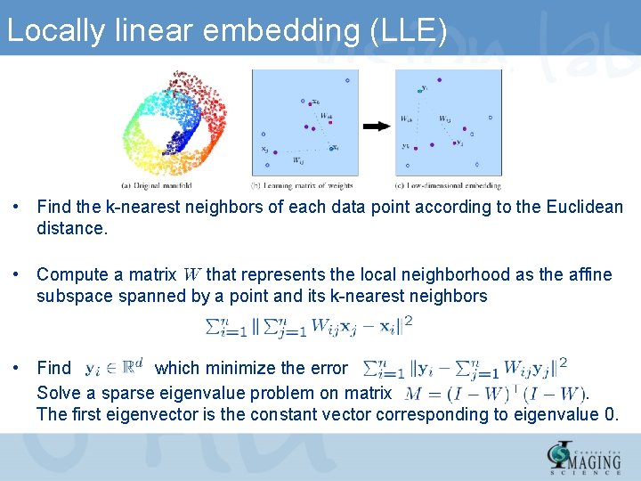
Locally linear embedding (LLE) • Find the k-nearest neighbors of each data point according to the Euclidean distance. • Compute a matrix that represents the local neighborhood as the affine subspace spanned by a point and its k-nearest neighbors • Find which minimize the error Solve a sparse eigenvalue problem on matrix. The first eigenvector is the constant vector corresponding to eigenvalue 0.

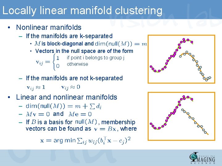
Locally linear manifold clustering • Nonlinear manifolds – If the manifolds are k-separated • is block-diagonal and • Vectors in the null space are of the form if point i belongs to group j otherwise – If the manifolds are not k-separated • Linear and nonlinear manifolds – – and – If is a basis for vectors can be found as , membership , where

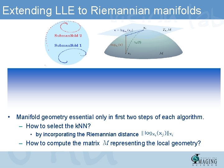
Extending LLE to Riemannian manifolds • Manifold geometry essential only in first two steps of each algorithm. – How to select the k. NN? • by incorporating the Riemannian distance – How to compute the matrix representing the local geometry?

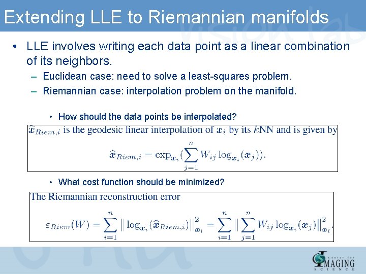
Extending LLE to Riemannian manifolds • LLE involves writing each data point as a linear combination of its neighbors. – Euclidean case: need to solve a least-squares problem. – Riemannian case: interpolation problem on the manifold. • How should the data points be interpolated? • What cost function should be minimized?

Part III: Applications in Computer Vision and Diffusion Tensor Imaging René Vidal Center for Imaging Science Institute for Computational Medicine Johns Hopkins University

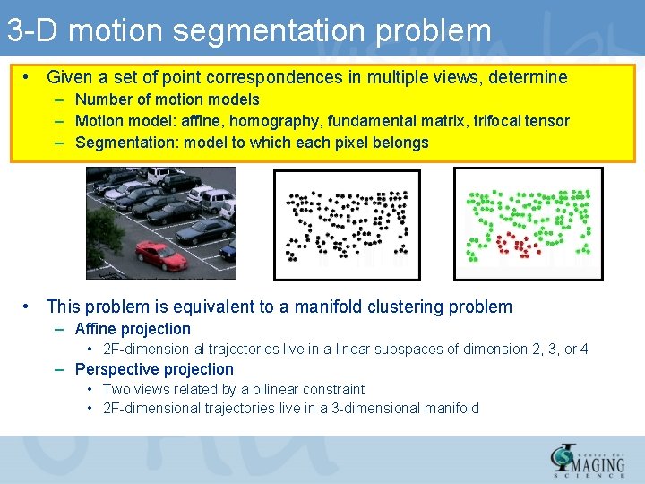
3 -D motion segmentation problem • Given a set of point correspondences in multiple views, determine – Number of motion models – Motion model: affine, homography, fundamental matrix, trifocal tensor – Segmentation: model to which each pixel belongs • This problem is equivalent to a manifold clustering problem – Affine projection • 2 F-dimension al trajectories live in a linear subspaces of dimension 2, 3, or 4 – Perspective projection • Two views related by a bilinear constraint • 2 F-dimensional trajectories live in a 3 -dimensional manifold

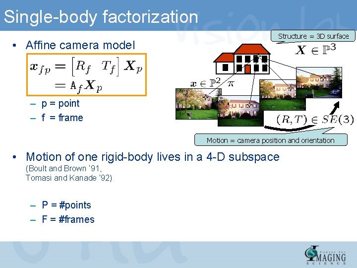
Single-body factorization • Affine camera model Structure = 3 D surface – p = point – f = frame Motion = camera position and orientation • Motion of one rigid-body lives in a 4 -D subspace (Boult and Brown ’ 91, Tomasi and Kanade ‘ 92) – P = #points – F = #frames

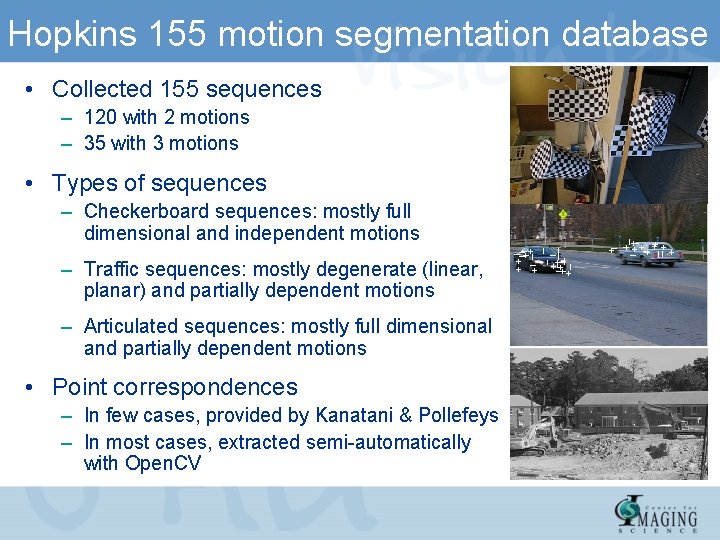
Hopkins 155 motion segmentation database • Collected 155 sequences – 120 with 2 motions – 35 with 3 motions • Types of sequences – Checkerboard sequences: mostly full dimensional and independent motions – Traffic sequences: mostly degenerate (linear, planar) and partially dependent motions – Articulated sequences: mostly full dimensional and partially dependent motions • Point correspondences – In few cases, provided by Kanatani & Pollefeys – In most cases, extracted semi-automatically with Open. CV

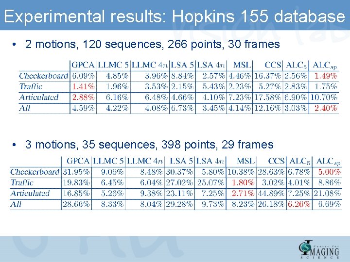
Experimental results: Hopkins 155 database • 2 motions, 120 sequences, 266 points, 30 frames • 3 motions, 35 sequences, 398 points, 29 frames

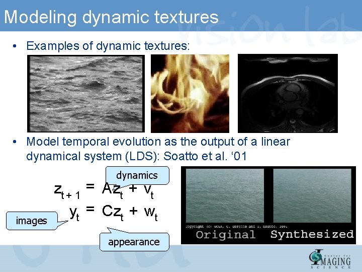
Modeling dynamic textures • Examples of dynamic textures: • Model temporal evolution as the output of a linear dynamical system (LDS): Soatto et al. ‘ 01 dynamics images zt + 1 = Azt + vt yt = Czt + wt appearance

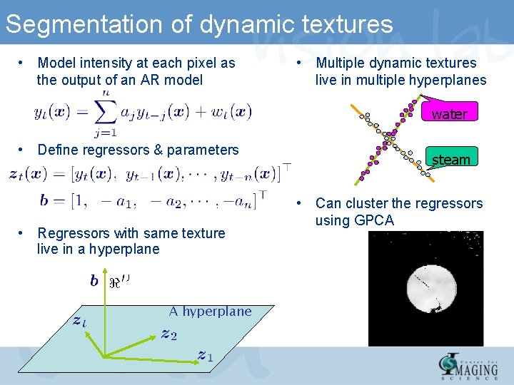
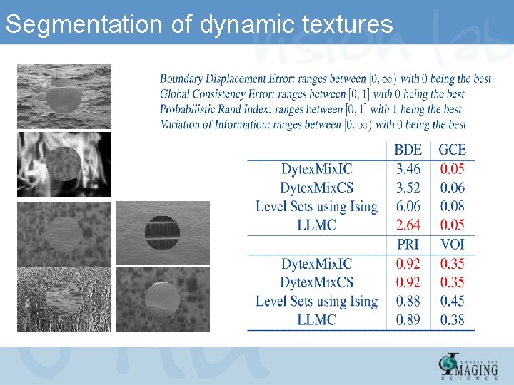
Segmentation of dynamic textures • Model intensity at each pixel as the output of an AR model • Multiple dynamic textures live in multiple hyperplanes water • Define regressors & parameters • Regressors with same texture live in a hyperplane A hyperplane steam • Can cluster the regressors using GPCA

Segmentation of dynamic textures

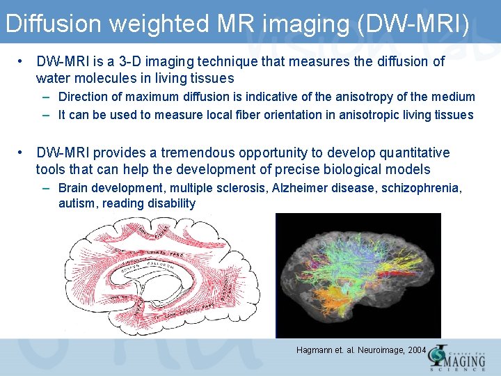
Diffusion weighted MR imaging (DW-MRI) • DW-MRI is a 3 -D imaging technique that measures the diffusion of water molecules in living tissues – Direction of maximum diffusion is indicative of the anisotropy of the medium – It can be used to measure local fiber orientation in anisotropic living tissues • DW-MRI provides a tremendous opportunity to develop quantitative tools that can help the development of precise biological models – Brain development, multiple sclerosis, Alzheimer disease, schizophrenia, autism, reading disability Hagmann et. al. Neuroimage, 2004

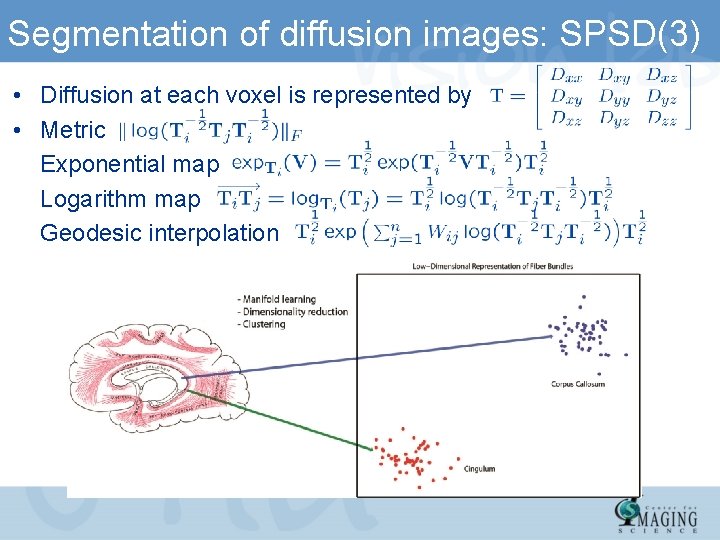
Segmentation of diffusion images: SPSD(3) • Diffusion at each voxel is represented by • Metric Exponential map Logarithm map Geodesic interpolation

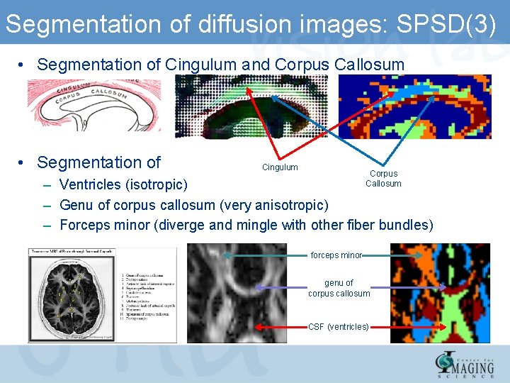
Segmentation of diffusion images: SPSD(3) • Segmentation of Cingulum and Corpus Callosum • Segmentation of Cingulum Corpus Callosum – Ventricles (isotropic) – Genu of corpus callosum (very anisotropic) – Forceps minor (diverge and mingle with other fiber bundles) forceps minor genu of corpus callosum CSF (ventricles)

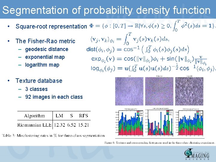
Segmentation of probability density function • Square-root representation • The Fisher-Rao metric – geodesic distance – exponential map – logarithm map • Texture database – 3 classes – 92 images in each class

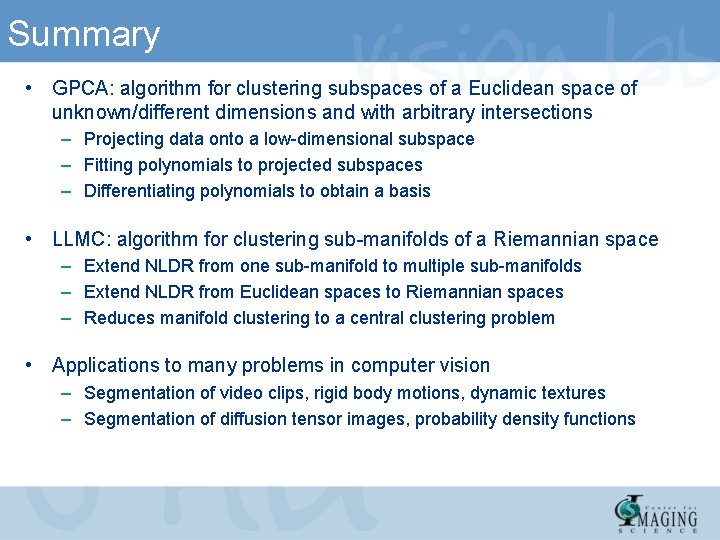
Summary • GPCA: algorithm for clustering subspaces of a Euclidean space of unknown/different dimensions and with arbitrary intersections – Projecting data onto a low-dimensional subspace – Fitting polynomials to projected subspaces – Differentiating polynomials to obtain a basis • LLMC: algorithm for clustering sub-manifolds of a Riemannian space – Extend NLDR from one sub-manifold to multiple sub-manifolds – Extend NLDR from Euclidean spaces to Riemannian spaces – Reduces manifold clustering to a central clustering problem • Applications to many problems in computer vision – Segmentation of video clips, rigid body motions, dynamic textures – Segmentation of diffusion tensor images, probability density functions

References: Springer-Verlag 2008

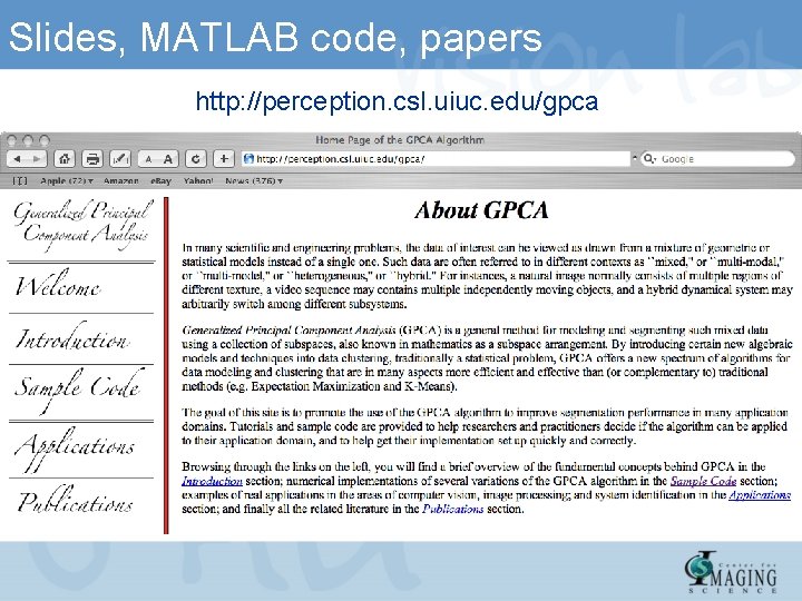
Slides, MATLAB code, papers http: //perception. csl. uiuc. edu/gpca

For more information, Vision Lab @ Johns Hopkins University Thank You! • • • NSF CNS-0809101 • NSF ISS-0447739 • ARL Robotics-CTA ONR N 00014 -05 -10836 • NSF CNS-0509101 JHU APL-934652 NIH RO 1 HL 082729 WSE-APL NIH-NHLBI