Managing Inventory 12 Power Point presentation to accompany

Managing Inventory 12 Power. Point presentation to accompany Heizer and Render Operations Management, Global Edition, Eleventh Edition Principles of Operations Management, Global Edition, Ninth Edition Power. Point slides by Jeff Heyl © 2014 Pearson Education 12 - 1

Outline 1. Types of Inventory 2. Functions of Inventory 3. ABC Analysis 4. Record Accuracy 5. Cycle Counting 6. Independent vs. Dependent Demand Inventory Control Systems © 2011 Pearson Education, Inc. publishing as Prentice Hall 12 - 2

Outline – Continued 7. Multi-Period Models Deterministic Inventory I. Fixed- Order Quantity Models ü Economic Model. ü Production Model. Order Quantity (EOQ) Quantity (POQ) ü Quantity Discount Model. II. Fixed-Time Period Models 8. Probabilistic Models and Safety Stock 9. Single-Period Inventory Model © 2011 Pearson Education, Inc. publishing as Prentice Hall 12 - 3

Amazon. com u Amazon. com started as a “virtual” retailer – no inventory, no warehouses, no overhead; just computers taking orders to be filled by others u Growth has forced Amazon. com to become a world leader in warehousing and inventory management © 2011 Pearson Education, Inc. publishing as Prentice Hall 12 - 4

Inventory Management The objective of inventory management is to strike a balance between inventory investment and customer service © 2011 Pearson Education, Inc. publishing as Prentice Hall 12 - 5

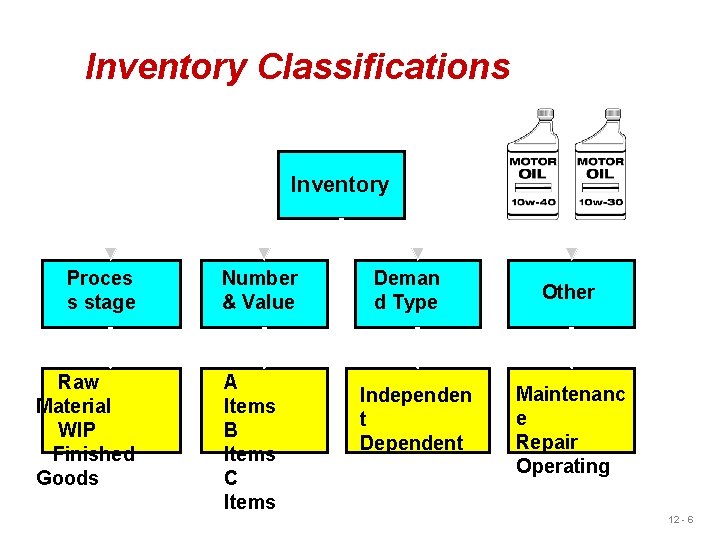
Inventory Classifications Inventory Proces s stage Raw Material WIP Finished Goods Number & Value A Items B Items C Items Deman d Type Independen t Dependent Other Maintenanc e Repair Operating 12 - 6

Functions of Inventory 1. To decouple various parts of the production process by covering delays 2. To protect the company against fluctuations in demand 3. To provide a selection for customers 4. To take advantage of quantity discounts 5. To hedge against inflation © 2011 Pearson Education, Inc. publishing as Prentice Hall 12 - 7

Problems Caused by Inventory u Inventory ties up working capital u Inventory takes up space u Inventory is prone to: u. Damage, Pilferage and Obsolescence u Inventory hides problems 12 - 8

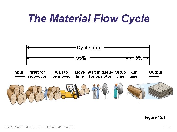
The Material Flow Cycle time 95% Input Wait for inspection Wait to be moved 5% Move Wait in queue Setup Run time for operator time Output Figure 12. 1 © 2011 Pearson Education, Inc. publishing as Prentice Hall 12 - 9

Important Issues in Inventory Management 1. Classifying inventory items 2. Keeping accurate inventory records © 2011 Pearson Education, Inc. publishing as Prentice Hall 12 - 10

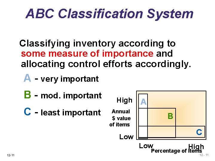
ABC Classification System Classifying inventory according to some measure of importance and allocating control efforts accordingly. A - very important B - mod. important C - least important High A Annual $ value of items B C Low 12 -11 High Percentage of Items 12 - 11

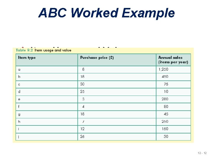
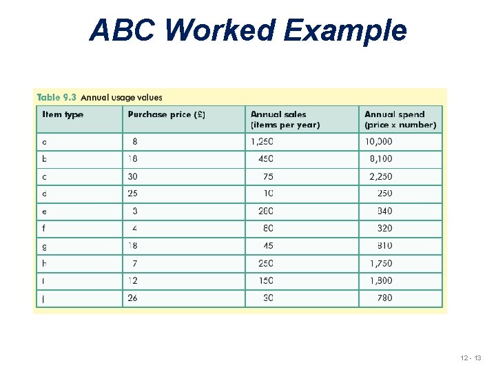
ABC Worked Example u Item Usage and Value 12 - 12

ABC Worked Example u Annual Usage Values 12 - 13

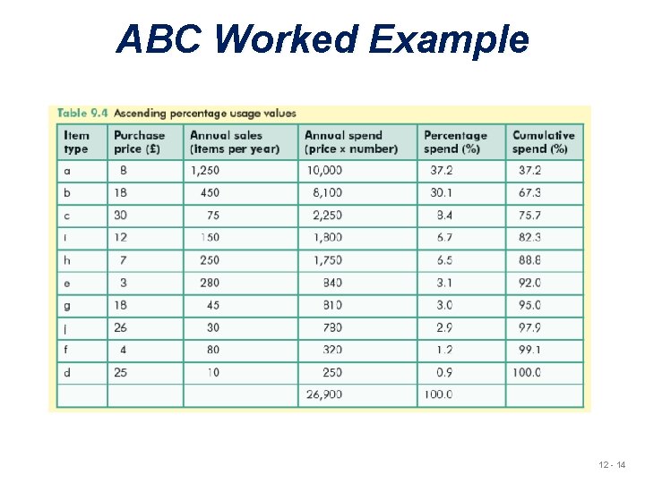
ABC Worked Example u Ascending Usage Values 12 - 14

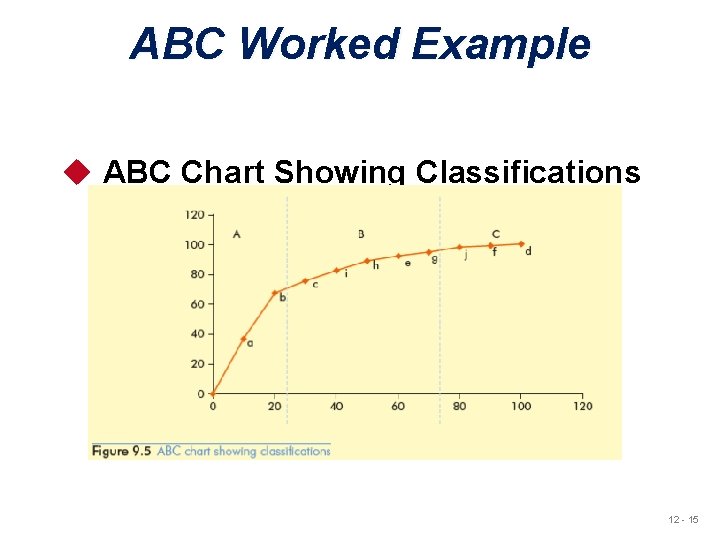
ABC Worked Example u ABC Chart Showing Classifications 12 - 15

ABC Classification System u Policies employed for A items may include u. More emphasis on supplier development u. Tighter physical inventory control u. More care in forecasting © 2011 Pearson Education, Inc. publishing as Prentice Hall 12 - 16

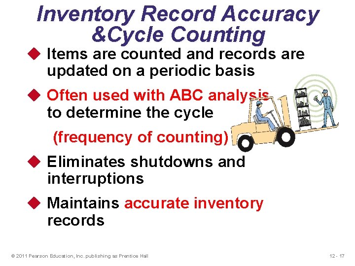
Inventory Record Accuracy &Cycle Counting u Items are counted and records are updated on a periodic basis u Often used with ABC analysis to determine the cycle (frequency of counting) u Eliminates shutdowns and interruptions u Maintains accurate inventory records © 2011 Pearson Education, Inc. publishing as Prentice Hall 12 - 17

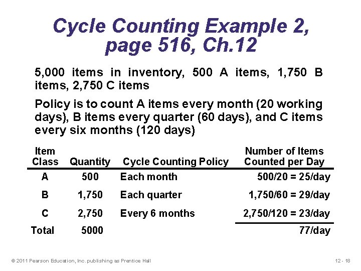
Cycle Counting Example 2, page 516, Ch. 12 5, 000 items in inventory, 500 A items, 1, 750 B items, 2, 750 C items Policy is to count A items every month (20 working days), B items every quarter (60 days), and C items every six months (120 days) Item Class Quantity A 500 Each month B 1, 750 Each quarter C 2, 750 Every 6 months Total 5000 Cycle Counting Policy © 2011 Pearson Education, Inc. publishing as Prentice Hall Number of Items Counted per Day 500/20 = 25/day 1, 750/60 = 29/day 2, 750/120 = 23/day 77/day 12 - 18

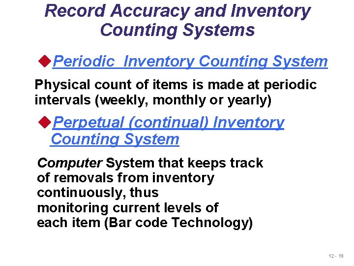
Record Accuracy and Inventory Counting Systems u. Periodic Inventory Counting System Physical count of items is made at periodic intervals (weekly, monthly or yearly) u. Perpetual (continual) Inventory Counting System Computer System that keeps track of removals from inventory continuously, thus monitoring current levels of each item (Bar code Technology) 12 - 19

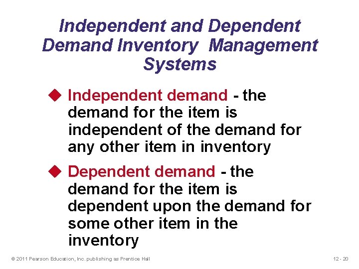
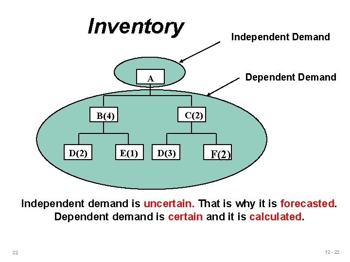
Independent and Dependent Demand Inventory Management Systems u Independent demand - the demand for the item is independent of the demand for any other item in inventory u Dependent demand - the demand for the item is dependent upon the demand for some other item in the inventory © 2011 Pearson Education, Inc. publishing as Prentice Hall 12 - 20

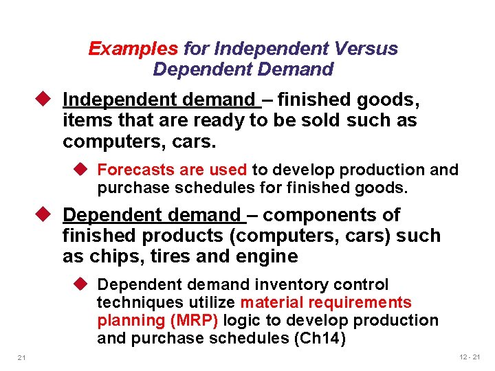
Examples for Independent Versus Dependent Demand u Independent demand – finished goods, items that are ready to be sold such as computers, cars. u Forecasts are used to develop production and purchase schedules for finished goods. u Dependent demand – components of finished products (computers, cars) such as chips, tires and engine u Dependent demand inventory control techniques utilize material requirements planning (MRP) logic to develop production and purchase schedules (Ch 14) 21 12 - 21

Inventory Independent Demand Dependent Demand A C(2) B(4) D(2) E(1) D(3) F(2) Independent demand is uncertain. That is why it is forecasted. Dependent demand is certain and it is calculated. 22 12 - 22

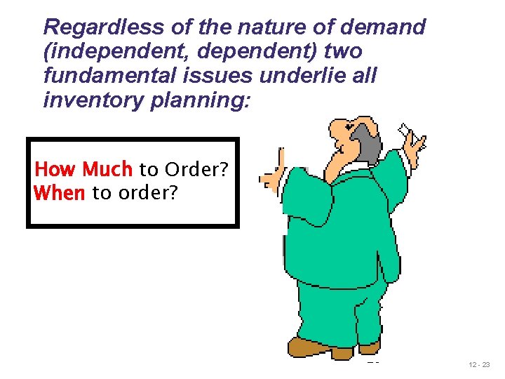
Regardless of the nature of demand (independent, dependent) two fundamental issues underlie all inventory planning: How Much to Order? When to order? 23 12 - 23

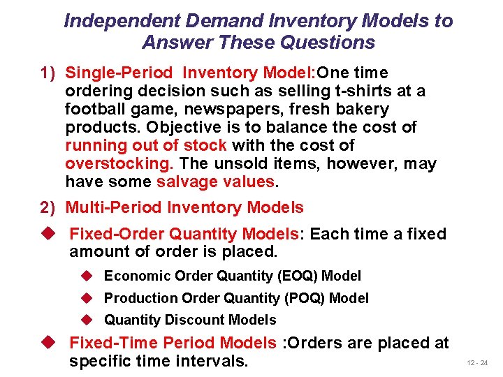
Independent Demand Inventory Models to Answer These Questions 1) Single-Period Inventory Model: One time ordering decision such as selling t-shirts at a football game, newspapers, fresh bakery products. Objective is to balance the cost of running out of stock with the cost of overstocking. The unsold items, however, may have some salvage values. 2) Multi-Period Inventory Models u Fixed-Order Quantity Models: Each time a fixed amount of order is placed. u Economic Order Quantity (EOQ) Model u Production Order Quantity (POQ) Model u Quantity Discount Models u Fixed-Time Period Models : Orders are placed at specific time intervals. 12 - 24

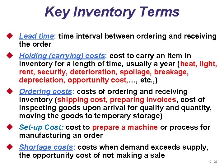
Key Inventory Terms u Lead time: time interval between ordering and receiving the order u Holding (carrying) costs: cost to carry an item in inventory for a length of time, usually a year (heat, light, rent, security, deterioration, spoilage, breakage, depreciation, opportunity cost, …, etc. , ) u Ordering costs: costs of ordering and receiving inventory (shipping cost, preparing invoices, cost of inspecting goods upon arrival for quality and quantity, moving the goods to temporary storage) u Set-up Cost: cost to prepare a machine or process for manufacturing an order u Shortage costs: costs when demand exceeds supply, the opportunity cost of not making a sale 12 - 25

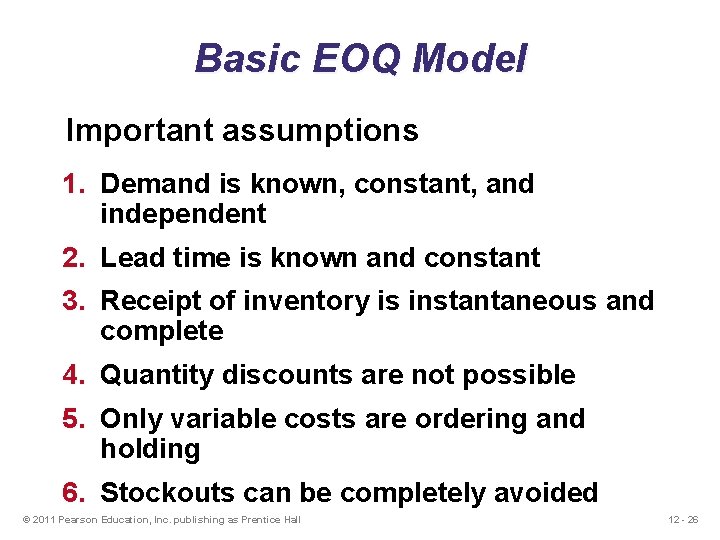
Basic EOQ Model Important assumptions 1. Demand is known, constant, and independent 2. Lead time is known and constant 3. Receipt of inventory is instantaneous and complete 4. Quantity discounts are not possible 5. Only variable costs are ordering and holding 6. Stockouts can be completely avoided © 2011 Pearson Education, Inc. publishing as Prentice Hall 12 - 26

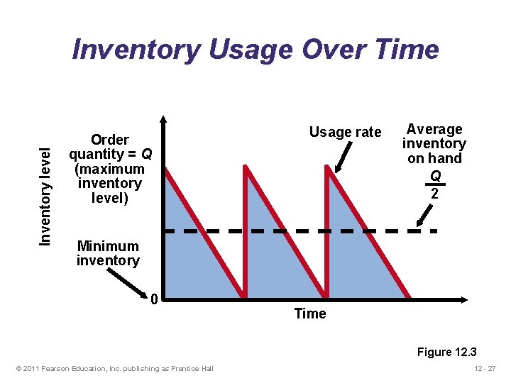
Inventory level Inventory Usage Over Time Order quantity = Q (maximum inventory level) Usage rate Average inventory on hand Q 2 Minimum inventory 0 Time Figure 12. 3 © 2011 Pearson Education, Inc. publishing as Prentice Hall 12 - 27

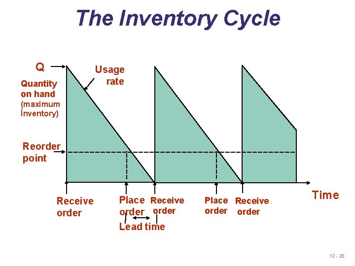
The Inventory Cycle Q Quantity on hand Usage rate (maximum İnventory) Reorder point Receive order Place Receive order Lead time Place Receive order Time 12 - 28

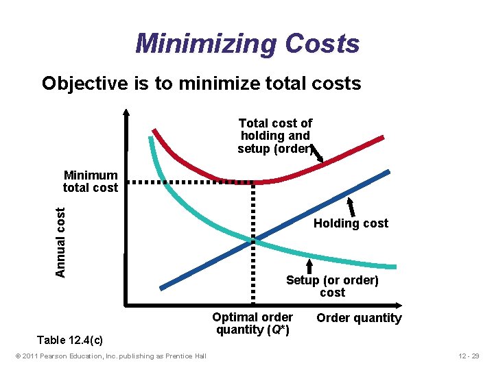
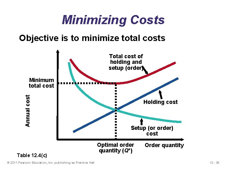
Minimizing Costs Objective is to minimize total costs Total cost of holding and setup (order) Annual cost Minimum total cost Table 12. 4(c) © 2011 Pearson Education, Inc. publishing as Prentice Hall Holding cost Setup (or order) cost Optimal order quantity (Q*) Order quantity 12 - 29

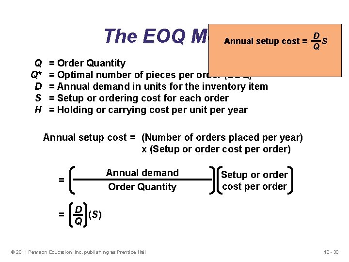
D The EOQ Model Annual setup cost = S Q Q Q* D S H = Order Quantity = Optimal number of pieces per order (EOQ) = Annual demand in units for the inventory item = Setup or ordering cost for each order = Holding or carrying cost per unit per year Annual setup cost = (Number of orders placed per year) x (Setup or order cost per order) Annual demand Order Quantity = = Setup or order cost per order D (S) Q © 2011 Pearson Education, Inc. publishing as Prentice Hall 12 - 30

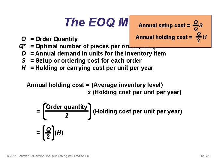
D The EOQ Model Annual setup cost = S Q Q Q* D S H Annual holding cost = = Order Quantity = Optimal number of pieces per order (EOQ) = Annual demand in units for the inventory item = Setup or ordering cost for each order = Holding or carrying cost per unit per year Q H 2 Annual holding cost = (Average inventory level) x (Holding cost per unit per year) = Order quantity (Holding cost per unit per year) 2 = Q (H) 2 © 2011 Pearson Education, Inc. publishing as Prentice Hall 12 - 31

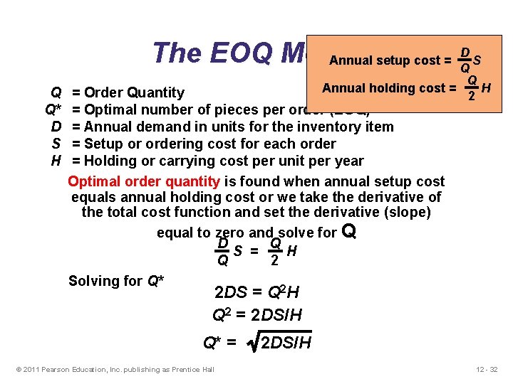
D The EOQ Model Annual setup cost = S Q Q Q* D S H Annual holding cost = = Order Quantity = Optimal number of pieces per order (EOQ) = Annual demand in units for the inventory item = Setup or ordering cost for each order = Holding or carrying cost per unit per year Optimal order quantity is found when annual setup cost equals annual holding cost or we take the derivative of the total cost function and set the derivative (slope) equal to zero and solve for Q D Q S = H Q 2 Solving for Q* 2 Q H 2 2 DS = Q H Q 2 = 2 DS/H Q* = © 2011 Pearson Education, Inc. publishing as Prentice Hall 2 DS/H 12 - 32

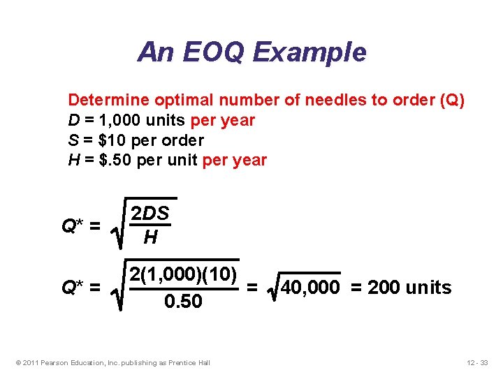
An EOQ Example Determine optimal number of needles to order (Q) D = 1, 000 units per year S = $10 per order H = $. 50 per unit per year Q* = 2 DS H Q* = 2(1, 000)(10) = 0. 50 © 2011 Pearson Education, Inc. publishing as Prentice Hall 40, 000 = 200 units 12 - 33

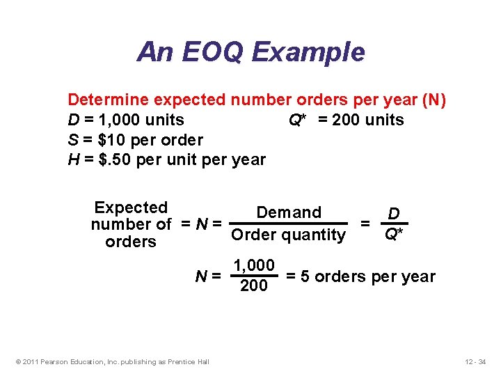
An EOQ Example Determine expected number orders per year (N) D = 1, 000 units Q* = 200 units S = $10 per order H = $. 50 per unit per year Expected Demand D number of = N = = Q* Order quantity orders 1, 000 N= = 5 orders per year 200 © 2011 Pearson Education, Inc. publishing as Prentice Hall 12 - 34

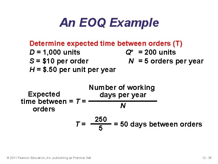
An EOQ Example Determine expected time between orders (T) D = 1, 000 units Q* = 200 units S = $10 per order N = 5 orders per year H = $. 50 per unit per year Expected time between = T = orders Number of working days per year T= © 2011 Pearson Education, Inc. publishing as Prentice Hall N 250 = 50 days between orders 5 12 - 35

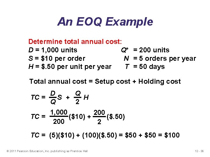
An EOQ Example Determine total annual cost: D = 1, 000 units Q* = 200 units S = $10 per order N = 5 orders per year H = $. 50 per unit per year T = 50 days Total annual cost = Setup cost + Holding cost TC = Q D S + H 2 Q 1, 000 200 TC = ($10) + ($. 50) 200 2 TC = (5)($10) + (100)($. 50) = $50 + $50 = $100 © 2011 Pearson Education, Inc. publishing as Prentice Hall 12 - 36

Robust Model u The EOQ model is robust u It works even if all parameters and assumptions are not met Because the total cost curve is relatively flat in the area of the EOQ © 2011 Pearson Education, Inc. publishing as Prentice Hall 12 - 37

Minimizing Costs Objective is to minimize total costs Total cost of holding and setup (order) Annual cost Minimum total cost Table 12. 4(c) © 2011 Pearson Education, Inc. publishing as Prentice Hall Holding cost Setup (or order) cost Optimal order quantity (Q*) Order quantity 12 - 38

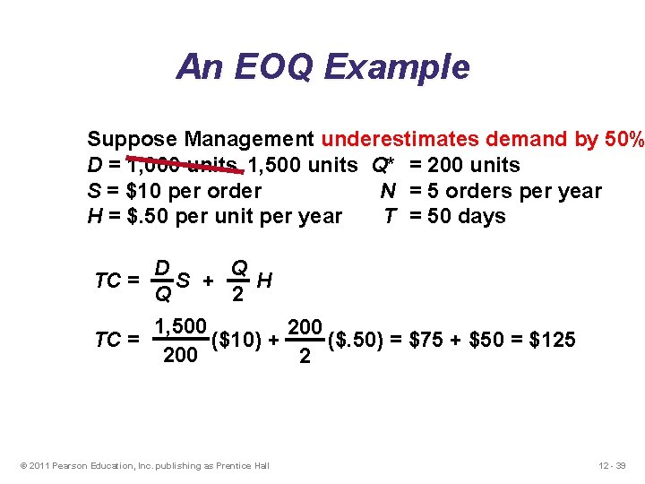
An EOQ Example Suppose Management underestimates demand by 50% D = 1, 000 units 1, 500 units Q* = 200 units S = $10 per order N = 5 orders per year H = $. 50 per unit per year T = 50 days Q D TC = S + H 2 Q TC = 1, 500 200 ($10) + ($. 50) = $75 + $50 = $125 200 2 © 2011 Pearson Education, Inc. publishing as Prentice Hall 12 - 39

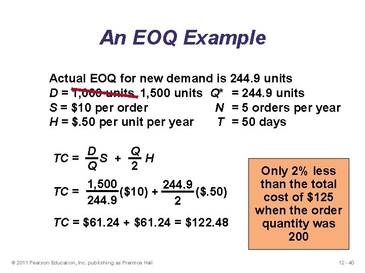
An EOQ Example Actual EOQ for new demand is 244. 9 units D = 1, 000 units 1, 500 units Q* = 244. 9 units S = $10 per order N = 5 orders per year H = $. 50 per unit per year T = 50 days Q D TC = S + H 2 Q TC = 1, 500 244. 9 ($10) + ($. 50) 244. 9 2 TC = $61. 24 + $61. 24 = $122. 48 © 2011 Pearson Education, Inc. publishing as Prentice Hall Only 2% less than the total cost of $125 when the order quantity was 200 12 - 40

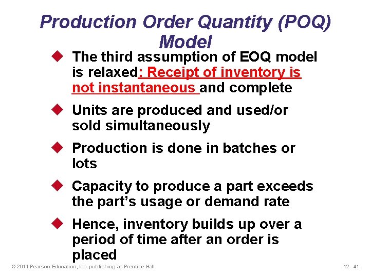
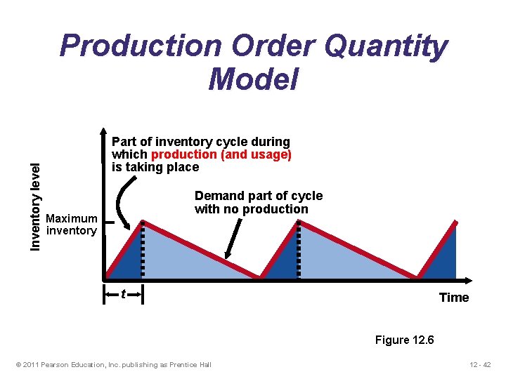
Production Order Quantity (POQ) Model u The third assumption of EOQ model is relaxed: Receipt of inventory is not instantaneous and complete u Units are produced and used/or sold simultaneously u Production is done in batches or lots u Capacity to produce a part exceeds the part’s usage or demand rate u Hence, inventory builds up over a period of time after an order is placed © 2011 Pearson Education, Inc. publishing as Prentice Hall 12 - 41

Inventory level Production Order Quantity Model Part of inventory cycle during which production (and usage) is taking place Demand part of cycle with no production Maximum inventory t Time Figure 12. 6 © 2011 Pearson Education, Inc. publishing as Prentice Hall 12 - 42

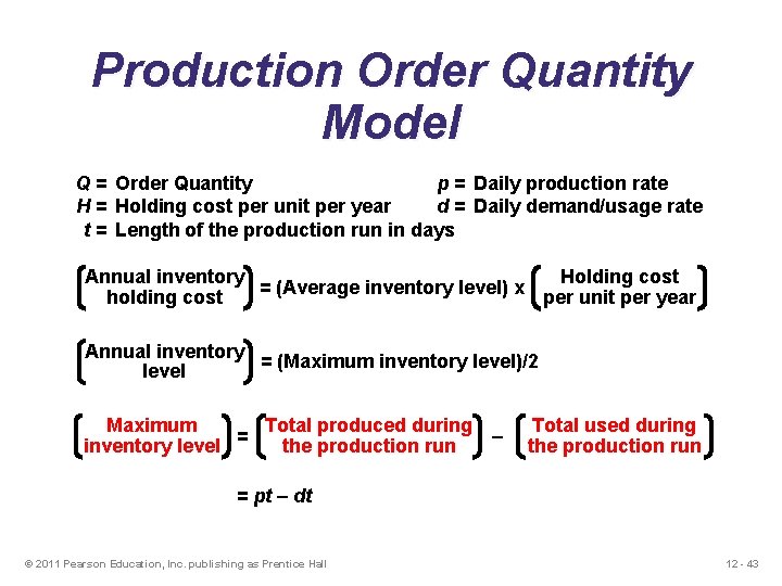
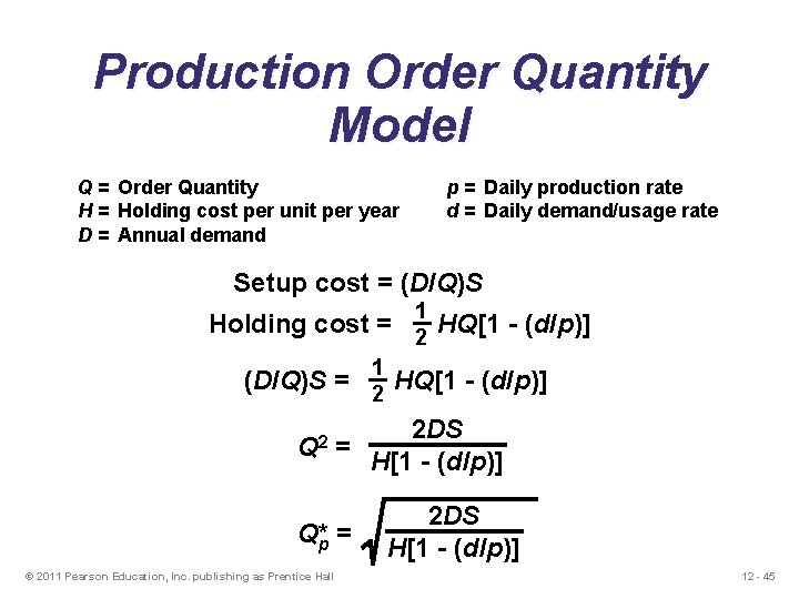
Production Order Quantity Model Q = Order Quantity p = Daily production rate H = Holding cost per unit per year d = Daily demand/usage rate t = Length of the production run in days Holding cost Annual inventory = (Average inventory level) x per unit per year holding cost Annual inventory = (Maximum inventory level)/2 level Total produced during Maximum = – the production run inventory level Total used during the production run = pt – dt © 2011 Pearson Education, Inc. publishing as Prentice Hall 12 - 43

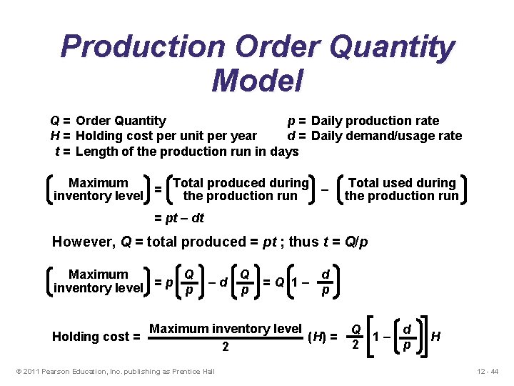
Production Order Quantity Model Q = Order Quantity p = Daily production rate H = Holding cost per unit per year d = Daily demand/usage rate t = Length of the production run in days Total produced during Maximum = – the production run inventory level Total used during the production run = pt – dt However, Q = total produced = pt ; thus t = Q/p Q Maximum = p inventory level p Holding cost = –d Q p =Q 1– d p Maximum inventory level (H) = 2 © 2011 Pearson Education, Inc. publishing as Prentice Hall Q d 1– 2 p H 12 - 44

Production Order Quantity Model Q = Order Quantity H = Holding cost per unit per year D = Annual demand p = Daily production rate d = Daily demand/usage rate Setup cost = (D/Q)S Holding cost = 1 2 HQ[1 - (d/p)] 1 (D/Q)S = 2 HQ[1 - (d/p)] 2 DS 2 Q = H[1 - (d/p)] Q*p = © 2011 Pearson Education, Inc. publishing as Prentice Hall 2 DS H[1 - (d/p)] 12 - 45

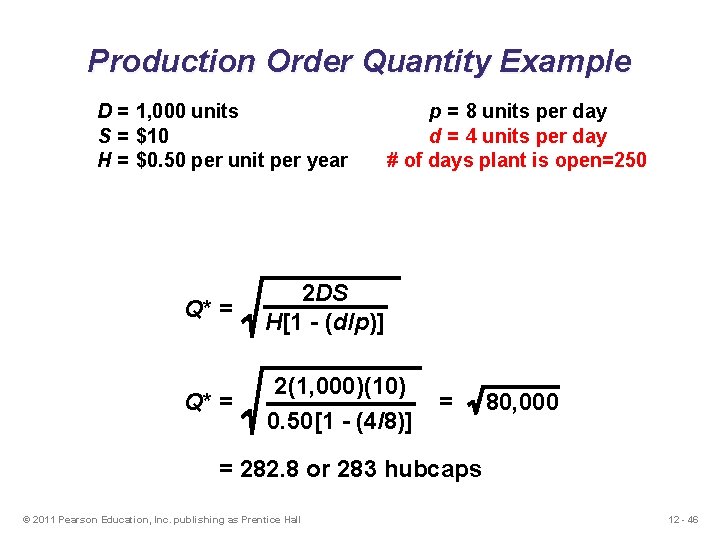
Production Order Quantity Example D = 1, 000 units S = $10 H = $0. 50 per unit per year p = 8 units per day d = 4 units per day # of days plant is open=250 Q* = 2 DS H[1 - (d/p)] Q* = 2(1, 000)(10) 0. 50[1 - (4/8)] = 80, 000 = 282. 8 or 283 hubcaps © 2011 Pearson Education, Inc. publishing as Prentice Hall 12 - 46

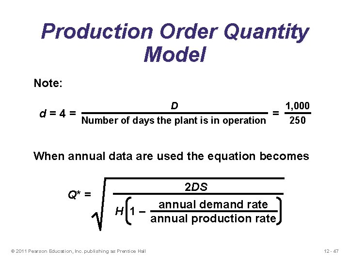
Production Order Quantity Model Note: d=4= D Number of days the plant is in operation = 1, 000 250 When annual data are used the equation becomes Q* = 2 DS annual demand rate H 1– annual production rate © 2011 Pearson Education, Inc. publishing as Prentice Hall 12 - 47

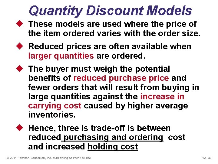
Quantity Discount Models u These models are used where the price of the item ordered varies with the order size. u Reduced prices are often available when larger quantities are ordered. u The buyer must weigh the potential benefits of reduced purchase price and fewer orders that will result from buying in large quantities against the increase in carrying cost caused by higher average inventories. u Hence, three is trade-off is between reduced purchasing and ordering cost and increased holding cost © 2011 Pearson Education, Inc. publishing as Prentice Hall 12 - 48

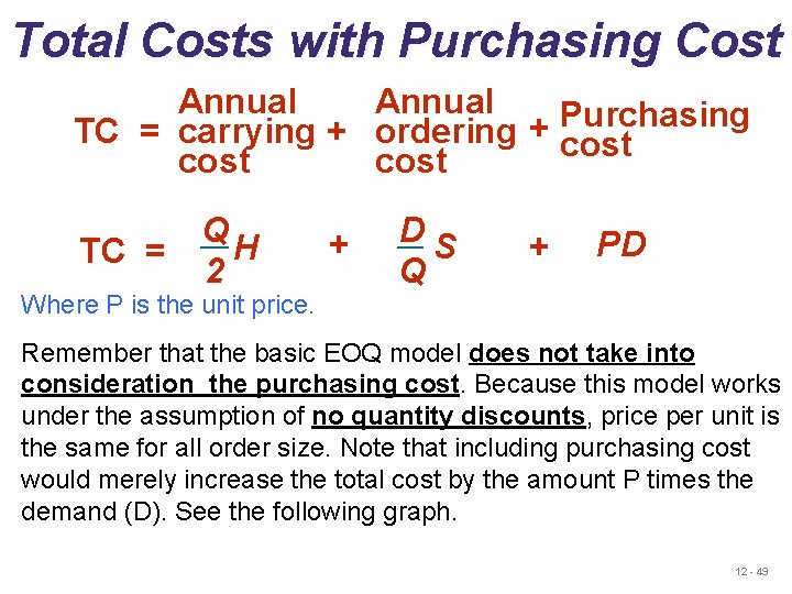
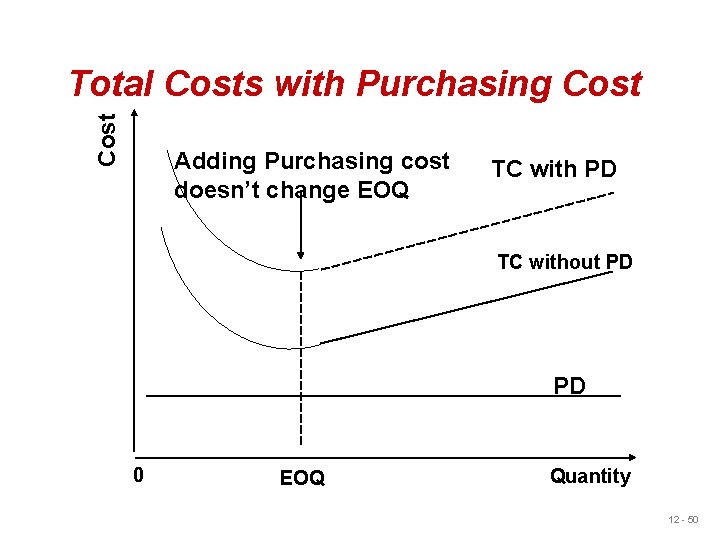
Total Costs with Purchasing Cost Annual Purchasing + TC = carrying + ordering cost Q H TC = 2 Where P is the unit price. + DS Q + PD Remember that the basic EOQ model does not take into consideration the purchasing cost. Because this model works under the assumption of no quantity discounts, price per unit is the same for all order size. Note that including purchasing cost would merely increase the total cost by the amount P times the demand (D). See the following graph. 12 - 49

Cost Total Costs with Purchasing Cost Adding Purchasing cost doesn’t change EOQ TC with PD TC without PD PD 0 EOQ Quantity 12 - 50

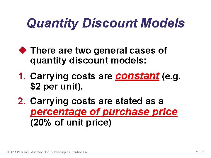
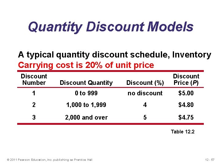
Quantity Discount Models u There are two general cases of quantity discount models: 1. Carrying costs are constant (e. g. $2 per unit). 2. Carrying costs are stated as a percentage of purchase price (20% of unit price) © 2011 Pearson Education, Inc. publishing as Prentice Hall 12 - 51

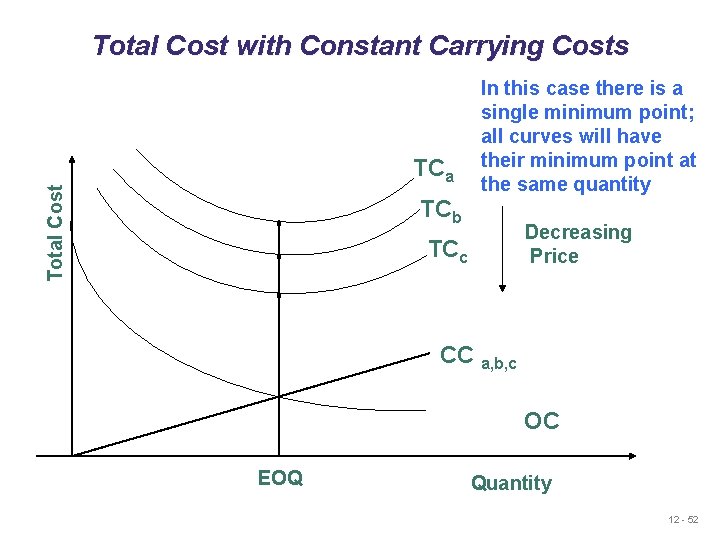
Total Cost with Constant Carrying Costs Total Cost TCa TCb In this case there is a single minimum point; all curves will have their minimum point at the same quantity Decreasing Price TCc CC a, b, c OC EOQ Quantity 12 - 52

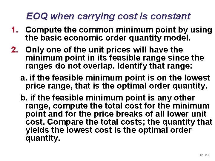
EOQ when carrying cost is constant 1. Compute the common minimum point by using the basic economic order quantity model. 2. Only one of the unit prices will have the minimum point in its feasible range since the ranges do not overlap. Identify that range: a. if the feasible minimum point is on the lowest price range, that is the optimal order quantity. b. if the feasible minimum point is any other range, compute the total cost for the minimum point and for the price breaks of all lower unit cost. Compare the total costs; the quantity that yields the lowest cost is the optimal order quantity. 12 - 53

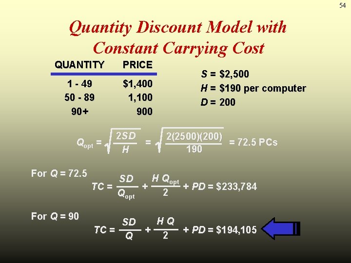
54 Quantity Discount Model with Constant Carrying Cost QUANTITY PRICE 1 - 49 50 - 89 90+ $1, 400 1, 100 900 Qopt = For Q = 72. 5 For Q = 90 2 S D = H S= H= D= $2, 500 $190 per computer 200 2(2500)(200) = 72. 5 PCs 190 H Qopt SD TC = + + PD = $233, 784 2 Qopt HQ SD TC = + + PD = $194, 105 2 Q

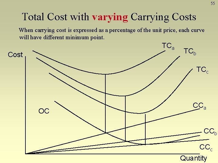
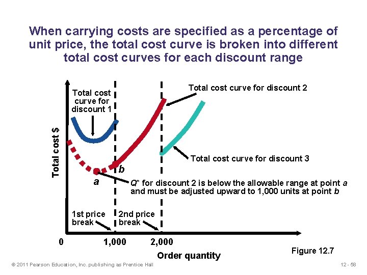
55 Total Cost with varying Carrying Costs When carrying cost is expressed as a percentage of the unit price, each curve will have different minimum point. TCa Cost TCb TCc OC CCa CCb CCc Quantity

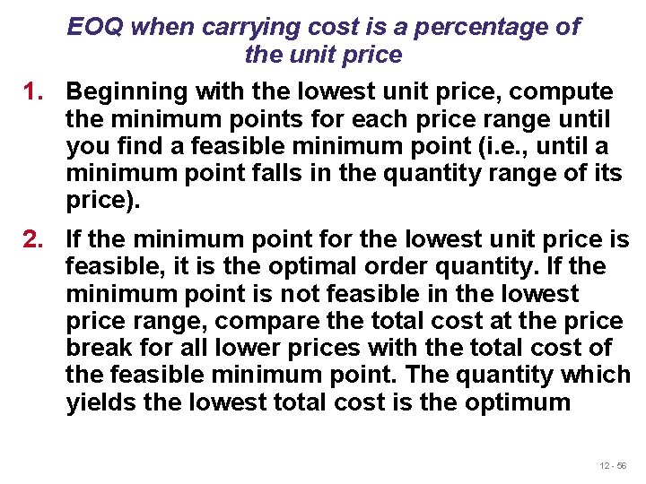
EOQ when carrying cost is a percentage of the unit price 1. Beginning with the lowest unit price, compute the minimum points for each price range until you find a feasible minimum point (i. e. , until a minimum point falls in the quantity range of its price). 2. If the minimum point for the lowest unit price is feasible, it is the optimal order quantity. If the minimum point is not feasible in the lowest price range, compare the total cost at the price break for all lower prices with the total cost of the feasible minimum point. The quantity which yields the lowest total cost is the optimum 12 - 56

Quantity Discount Models A typical quantity discount schedule, Inventory Carrying cost is 20% of unit price Discount Number Discount Quantity Discount (%) Discount Price (P) 1 0 to 999 no discount $5. 00 2 1, 000 to 1, 999 4 $4. 80 3 2, 000 and over 5 $4. 75 Table 12. 2 © 2011 Pearson Education, Inc. publishing as Prentice Hall 12 - 57

When carrying costs are specified as a percentage of unit price, the total cost curve is broken into different total cost curves for each discount range Total cost curve for discount 2 Total cost $ Total cost curve for discount 1 Total cost curve for discount 3 b a Q* for discount 2 is below the allowable range at point a and must be adjusted upward to 1, 000 units at point b 1 st price break 0 2 nd price break 1, 000 2, 000 Order quantity © 2011 Pearson Education, Inc. publishing as Prentice Hall Figure 12. 7 12 - 58

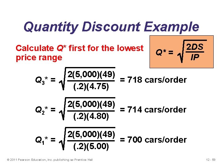
Quantity Discount Example Calculate Q* first for the lowest price range Q* = 2 DS IP Q 3* = 2(5, 000)(49) = 718 cars/order (. 2)(4. 75) Q 2* = 2(5, 000)(49) = 714 cars/order (. 2)(4. 80) Q 1* = 2(5, 000)(49) = 700 cars/order (. 2)(5. 00) © 2011 Pearson Education, Inc. publishing as Prentice Hall 12 - 59

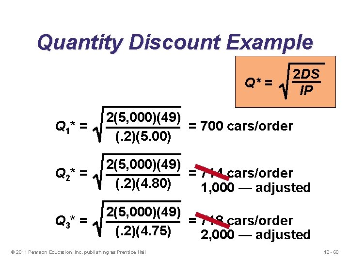
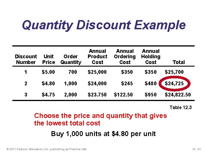
Quantity Discount Example Q* = 2 DS IP Q 1* = 2(5, 000)(49) = 700 cars/order (. 2)(5. 00) Q 2* = 2(5, 000)(49) = 714 cars/order (. 2)(4. 80) 1, 000 — adjusted Q 3* = 2(5, 000)(49) = 718 cars/order (. 2)(4. 75) 2, 000 — adjusted © 2011 Pearson Education, Inc. publishing as Prentice Hall 12 - 60

Quantity Discount Example Order Quantity Annual Product Cost Annual Ordering Cost Annual Holding Cost Discount Number Unit Price 1 $5. 00 700 $25, 000 $350 $25, 700 2 $4. 80 1, 000 $245 $480 $24, 725 3 $4. 75 2, 000 $23. 750 $122. 50 $950 $24, 822. 50 Total Table 12. 3 Choose the price and quantity that gives the lowest total cost Buy 1, 000 units at $4. 80 per unit © 2011 Pearson Education, Inc. publishing as Prentice Hall 12 - 61

When to Reorder with EOQ Ordering u The EOQ models answer the equation of how much to order, but not the question of when to order. The reorder point occurs when the quantity on hand drops to predetermined amount. u That amount generally includes expected demand during lead time. u In order to know when the reorder point has been reached, a perpetual inventory is required. u The goal of ordering is to place an order when the amount of inventory on hand is sufficient to satisfy demand during the time it takes to receive that order (i. e. , lead time) 12 - 62

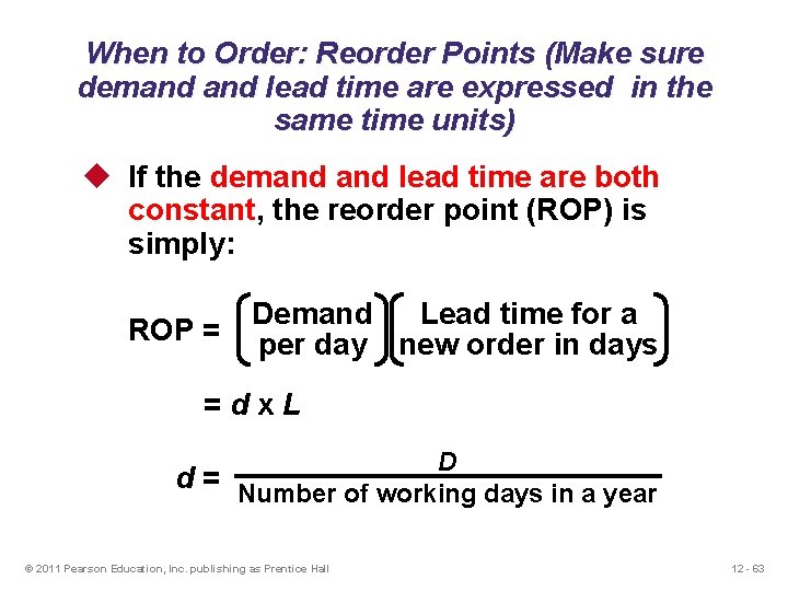
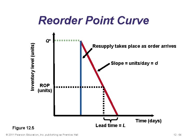
When to Order: Reorder Points (Make sure demand lead time are expressed in the same time units) u If the demand lead time are both constant, the reorder point (ROP) is simply: ROP = Lead time for a Demand per day new order in days =dx. L D d = Number of working days in a year © 2011 Pearson Education, Inc. publishing as Prentice Hall 12 - 63

Inventory level (units) Reorder Point Curve Q* Resupply takes place as order arrives Slope = units/day = d ROP (units) Figure 12. 5 © 2011 Pearson Education, Inc. publishing as Prentice Hall Lead time = L Time (days) 12 - 64

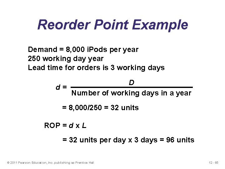
Reorder Point Example Demand = 8, 000 i. Pods per year 250 working day year Lead time for orders is 3 working days D d= Number of working days in a year = 8, 000/250 = 32 units ROP = d x L = 32 units per day x 3 days = 96 units © 2011 Pearson Education, Inc. publishing as Prentice Hall 12 - 65

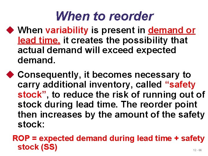
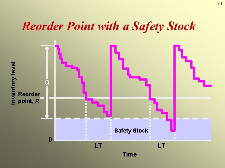
When to reorder u When variability is present in demand or lead time, it creates the possibility that actual demand will exceed expected demand. u Consequently, it becomes necessary to carry additional inventory, called “safety stock”, to reduce the risk of running out of stock during lead time. The reorder point then increases by the amount of the safety stock: ROP = expected demand during lead time + safety stock (SS) 12 - 66

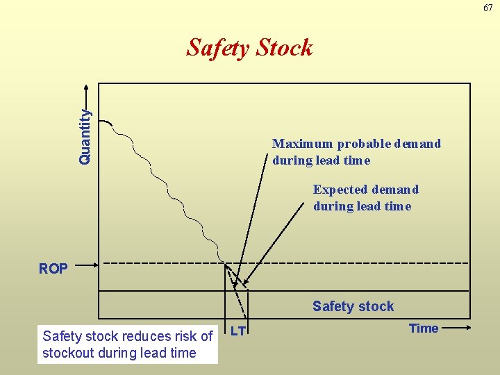
67 Quantity Safety Stock Maximum probable demand during lead time Expected demand during lead time ROP Safety stock reduces risk of stockout during lead time LT Time

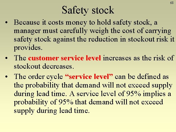
Safety stock 68 • Because it costs money to hold safety stock, a manager must carefully weigh the cost of carrying safety stock against the reduction in stockout risk it provides. • The customer service level increases as the risk of stockout decreases. • The order cycle “service level” can be defined as the probability that demand will not exceed supply during lead time. A service level of 95% implies a probability of 95% that demand will not exceed supply during lead time.

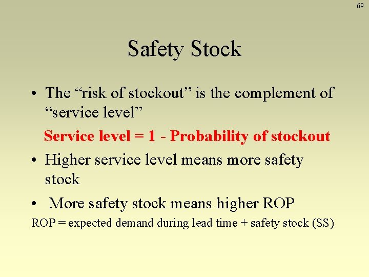
69 Safety Stock • The “risk of stockout” is the complement of “service level” Service level = 1 - Probability of stockout • Higher service level means more safety stock • More safety stock means higher ROP = expected demand during lead time + safety stock (SS)

70 Inventory level Reorder Point with a Safety Stock Q Reorder point, R Safety Stock 0 LT LT Time

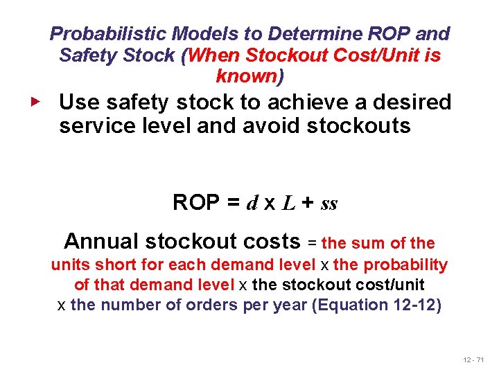
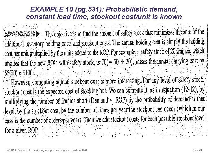
Probabilistic Models to Determine ROP and Safety Stock (When Stockout Cost/Unit is known) ▶ Use safety stock to achieve a desired service level and avoid stockouts ROP = d x L + ss Annual stockout costs = the sum of the units short for each demand level x the probability of that demand level x the stockout cost/unit x the number of orders per year (Equation 12 -12) 12 - 71

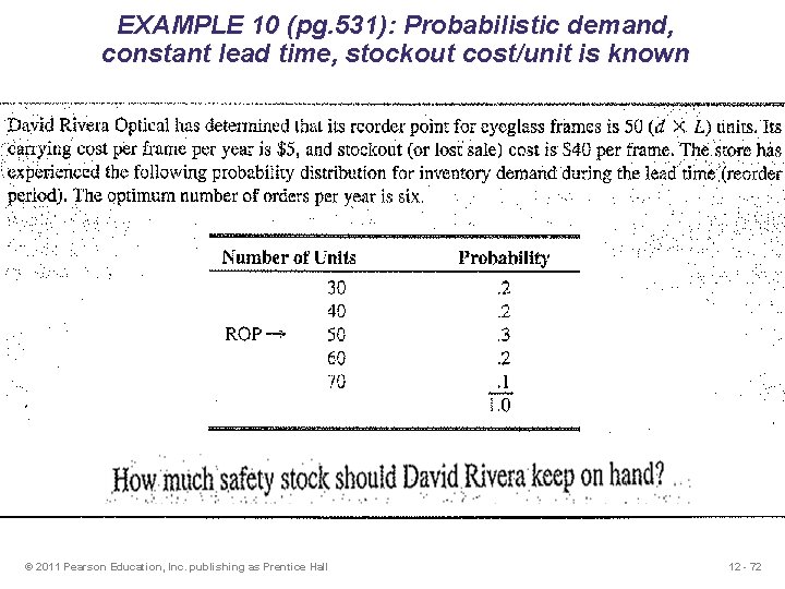
EXAMPLE 10 (pg. 531): Probabilistic demand, constant lead time, stockout cost/unit is known © 2011 Pearson Education, Inc. publishing as Prentice Hall 12 - 72

EXAMPLE 10 (pg. 531): Probabilistic demand, constant lead time, stockout cost/unit is known © 2011 Pearson Education, Inc. publishing as Prentice Hall 12 - 73

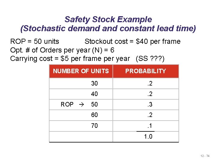
Safety Stock Example (Stochastic demand constant lead time) ROP = 50 units Stockout cost = $40 per frame Opt. # of Orders per year (N) = 6 Carrying cost = $5 per frame per year (SS ? ? ? ) NUMBER OF UNITS ROP PROBABILITY 30 . 2 40 . 2 50 . 3 60 . 2 70 . 1 1. 0 12 - 74

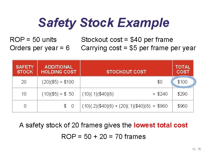
Safety Stock Example ROP = 50 units Orders per year = 6 Stockout cost = $40 per frame Carrying cost = $5 per frame per year SAFETY STOCK ADDITIONAL HOLDING COST 20 (20)($5) = $100 10 (10)($5) = $ 50 0 $ 0 TOTAL COST STOCKOUT COST $0 $100 = $240 $290 (10)(. 2)($40)(6) + (20)(. 1)($40)(6) = $960 (10)(. 1)($40)(6) A safety stock of 20 frames gives the lowest total cost ROP = 50 + 20 = 70 frames 12 - 75

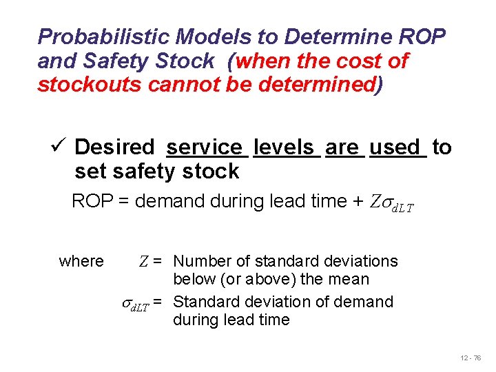
Probabilistic Models to Determine ROP and Safety Stock (when the cost of stockouts cannot be determined) ü Desired service levels are used to set safety stock ROP = demand during lead time + Zsd. LT where Z = Number of standard deviations below (or above) the mean sd. LT = Standard deviation of demand during lead time 12 - 76

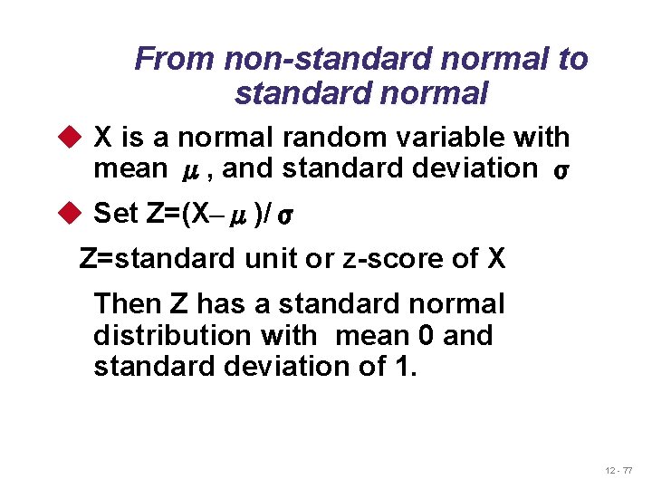
From non-standard normal to standard normal u X is a normal random variable with mean μ, and standard deviation σ u Set Z=(X–μ)/σ Z=standard unit or z-score of X Then Z has a standard normal distribution with mean 0 and standard deviation of 1. 12 - 77

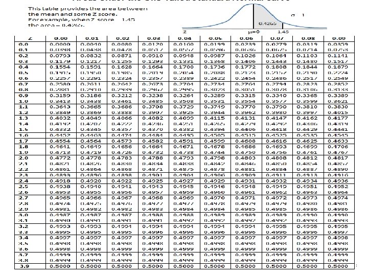
© 2011 Pearson Education, Inc. publishing as Prentice Hall 12 - 78

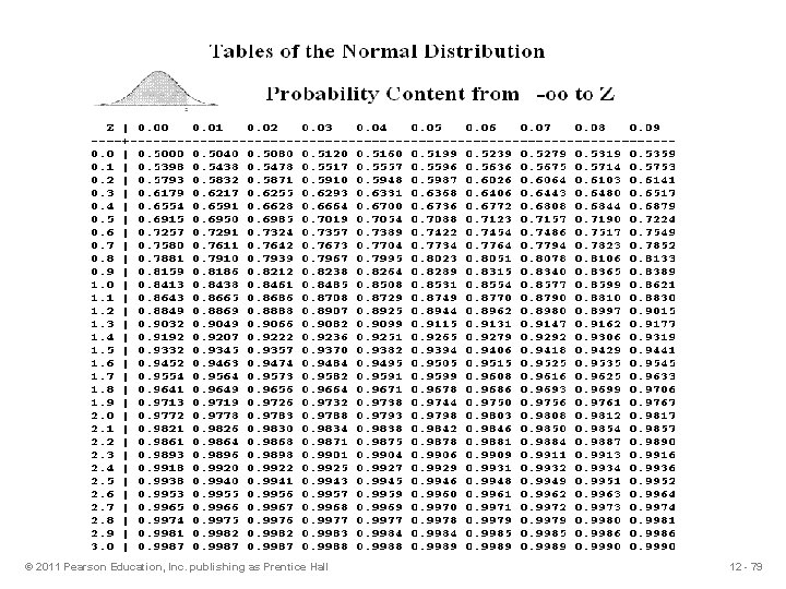
© 2011 Pearson Education, Inc. publishing as Prentice Hall 12 - 79

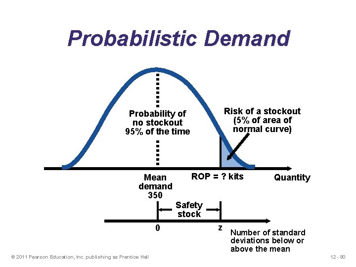
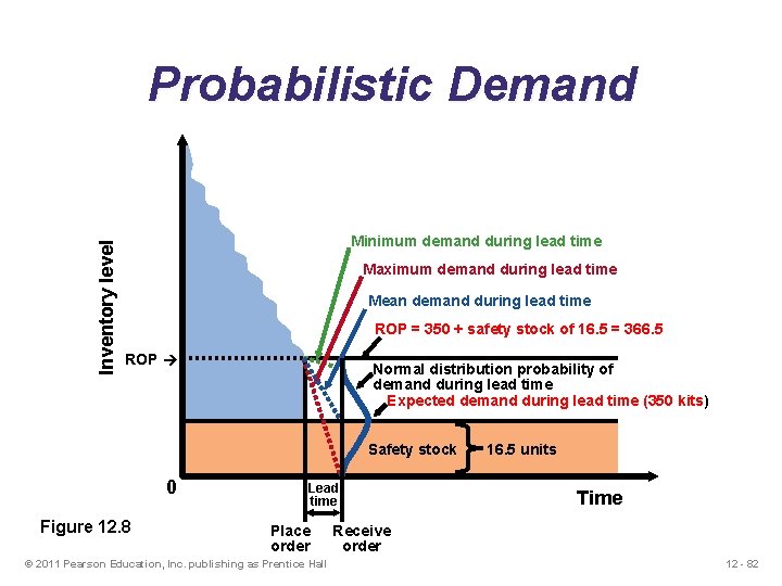
Probabilistic Demand Risk of a stockout (5% of area of normal curve) Probability of no stockout 95% of the time Mean demand 350 0 © 2011 Pearson Education, Inc. publishing as Prentice Hall ROP = ? kits Quantity Safety stock z Number of standard deviations below or above the mean 12 - 80

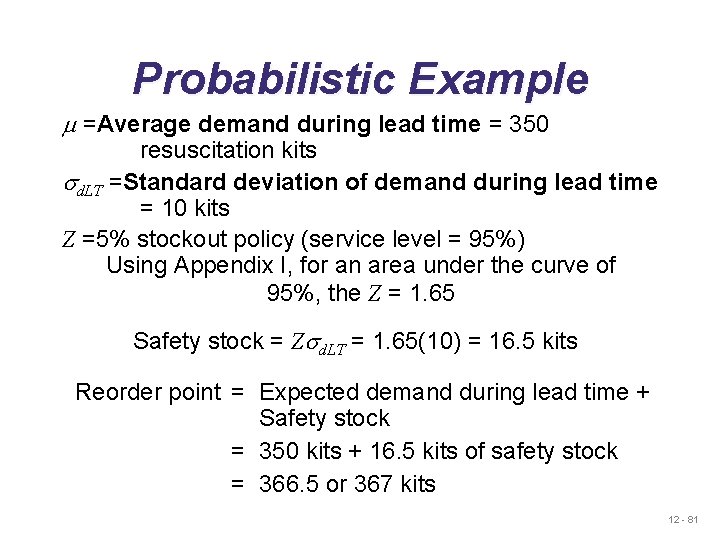
Probabilistic Example m =Average demand during lead time = 350 resuscitation kits sd. LT =Standard deviation of demand during lead time = 10 kits Z =5% stockout policy (service level = 95%) Using Appendix I, for an area under the curve of 95%, the Z = 1. 65 Safety stock = Zsd. LT = 1. 65(10) = 16. 5 kits Reorder point = Expected demand during lead time + Safety stock = 350 kits + 16. 5 kits of safety stock = 366. 5 or 367 kits 12 - 81

Inventory level Probabilistic Demand Minimum demand during lead time Maximum demand during lead time Mean demand during lead time ROP = 350 + safety stock of 16. 5 = 366. 5 ROP Normal distribution probability of demand during lead time Expected demand during lead time (350 kits) Safety stock 0 Figure 12. 8 Lead time Place order © 2011 Pearson Education, Inc. publishing as Prentice Hall 16. 5 units Time Receive order 12 - 82

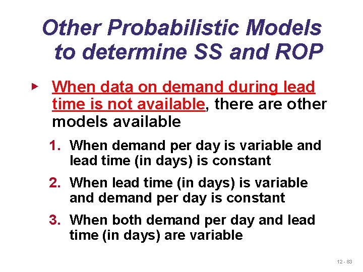
Other Probabilistic Models to determine SS and ROP ▶ When data on demand during lead time is not available, there are other models available 1. When demand per day is variable and lead time (in days) is constant 2. When lead time (in days) is variable and demand per day is constant 3. When both demand per day and lead time (in days) are variable 12 - 83

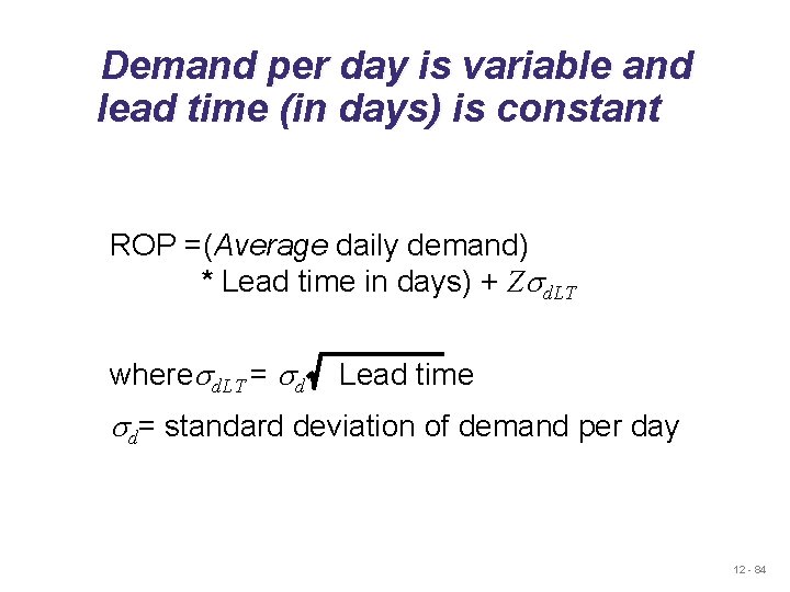
Demand per day is variable and lead time (in days) is constant ROP =(Average daily demand) * Lead time in days) + Zsd. LT wheresd. LT = sd Lead time sd= standard deviation of demand per day 12 - 84

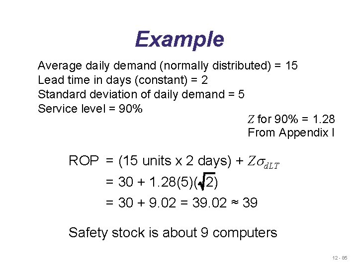
Example Average daily demand (normally distributed) = 15 Lead time in days (constant) = 2 Standard deviation of daily demand = 5 Service level = 90% Z for 90% = 1. 28 From Appendix I ROP = (15 units x 2 days) + Zsd. LT = 30 + 1. 28(5)( 2) = 30 + 9. 02 = 39. 02 ≈ 39 Safety stock is about 9 computers 12 - 85

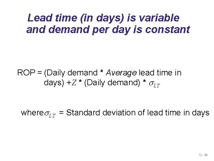
Lead time (in days) is variable and demand per day is constant ROP = (Daily demand * Average lead time in days) +Z * (Daily demand) * s. LT wheres. LT = Standard deviation of lead time in days 12 - 86

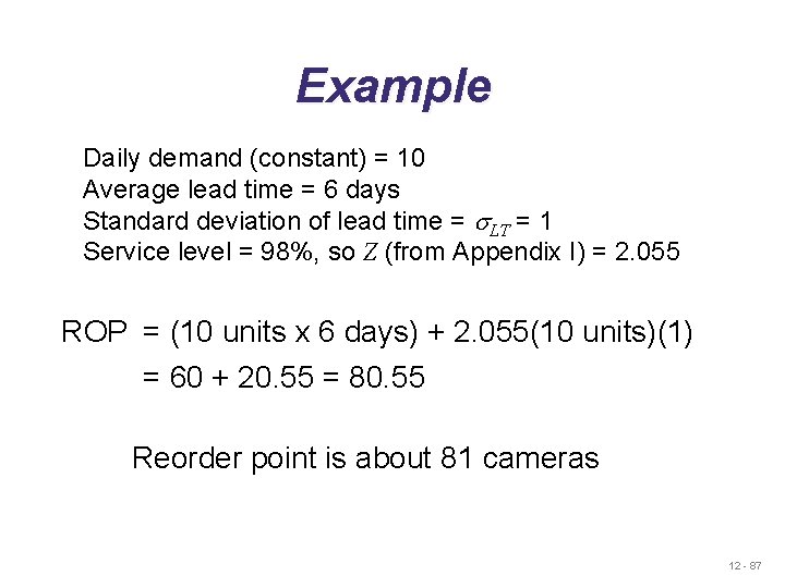
Example Daily demand (constant) = 10 Average lead time = 6 days Standard deviation of lead time = s. LT = 1 Service level = 98%, so Z (from Appendix I) = 2. 055 ROP = (10 units x 6 days) + 2. 055(10 units)(1) = 60 + 20. 55 = 80. 55 Reorder point is about 81 cameras 12 - 87

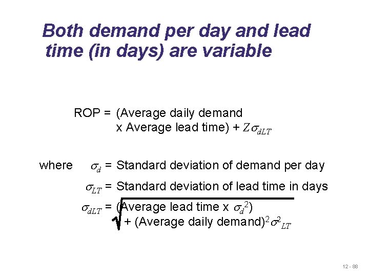
Both demand per day and lead time (in days) are variable ROP = (Average daily demand x Average lead time) + Zsd. LT where sd = Standard deviation of demand per day s. LT = Standard deviation of lead time in days sd. LT = (Average lead time x sd 2) + (Average daily demand)2 s 2 LT 12 - 88

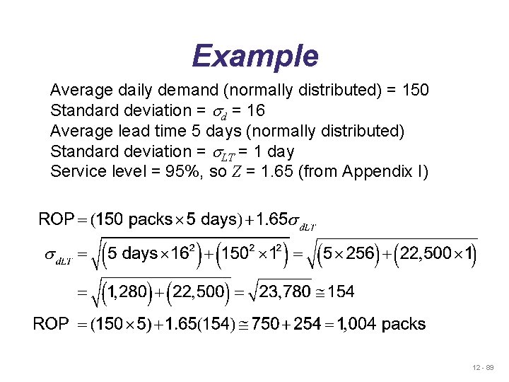
Example Average daily demand (normally distributed) = 150 Standard deviation = sd = 16 Average lead time 5 days (normally distributed) Standard deviation = s. LT = 1 day Service level = 95%, so Z = 1. 65 (from Appendix I) 12 - 89

Single-Period Inventory Model Used to handle ordering of perishables (fresh fruits, flowers) and other items with limited useful lives (newspapers, spare parts for specialized equipment). 12 - 90

Single-Period Inventory Model u In a single-period model, items are received in the beginning of a period and sold during the same period. The unsold items are not carried over to the next period. u The unsold items may be a total waste, or sold at a reduced price, or returned to the producer at some price less than the original purchase price. u The revenue generated by the unsold items is called the salvage value. 12 - 91

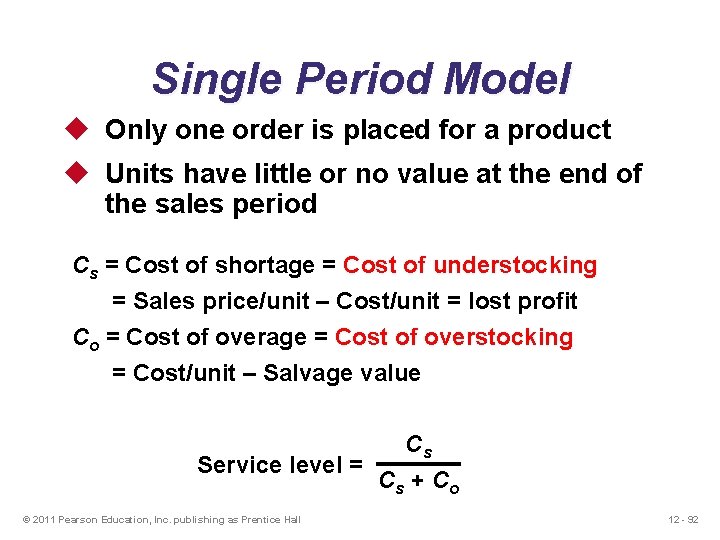
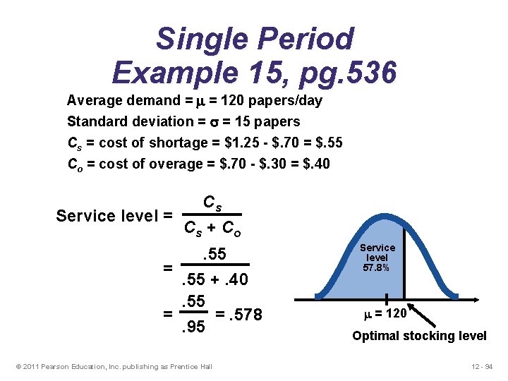
Single Period Model u Only one order is placed for a product u Units have little or no value at the end of the sales period Cs = Cost of shortage = Cost of understocking = Sales price/unit – Cost/unit = lost profit Co = Cost of overage = Cost of overstocking = Cost/unit – Salvage value Cs Service level = Cs + Co © 2011 Pearson Education, Inc. publishing as Prentice Hall 12 - 92

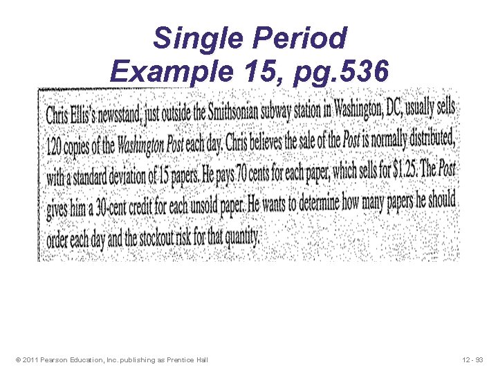
Single Period Example 15, pg. 536 © 2011 Pearson Education, Inc. publishing as Prentice Hall 12 - 93

Single Period Example 15, pg. 536 Average demand = = 120 papers/day Standard deviation = = 15 papers Cs = cost of shortage = $1. 25 - $. 70 = $. 55 Co = cost of overage = $. 70 - $. 30 = $. 40 Cs Service level = Cs + Co. 55 =. 55 +. 40. 55 = =. 578. 95 © 2011 Pearson Education, Inc. publishing as Prentice Hall Service level 57. 8% = 120 Optimal stocking level 12 - 94

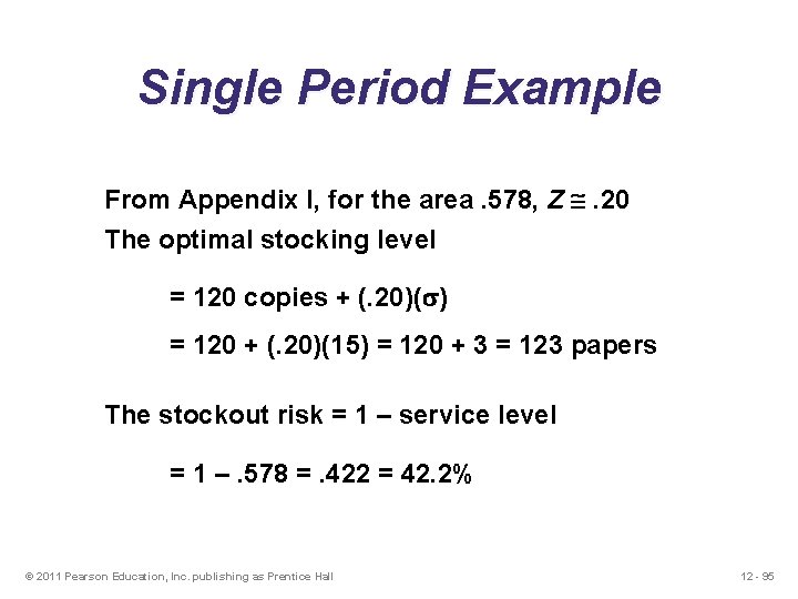
Single Period Example From Appendix I, for the area. 578, Z . 20 The optimal stocking level = 120 copies + (. 20)( ) = 120 + (. 20)(15) = 120 + 3 = 123 papers The stockout risk = 1 – service level = 1 –. 578 =. 422 = 42. 2% © 2011 Pearson Education, Inc. publishing as Prentice Hall 12 - 95

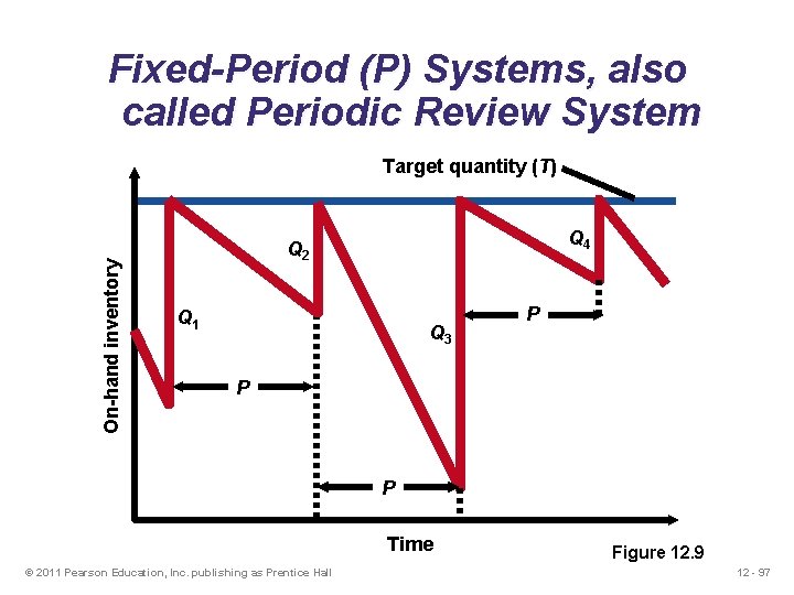
Fixed-Period (P) Systems ▶ Orders placed at the end of a fixed period ▶ Inventory counted only at the end of period ▶ Order brings inventory up to target level ▶ Only relevant costs are ordering and holding ▶ Lead times are known and constant ▶ Items are independent of one another 12 - 96

Fixed-Period (P) Systems, also called Periodic Review System On-hand inventory Target quantity (T) Q 4 Q 2 Q 1 Q 3 P P P Time © 2011 Pearson Education, Inc. publishing as Prentice Hall Figure 12. 9 12 - 97

Fixed-Period Systems ▶ Inventory is only counted at each review period ▶ May be scheduled at convenient times ▶ Appropriate in routine situations ▶ May result in stockouts between periods ▶ May require increased safety stock 12 - 98