Managerial Economics eighth edition Thomas Maurice Chapter 9

Managerial Economics eighth edition Thomas Maurice Chapter 9 Production & Cost in the Long Run Mc. Graw-Hill/Irwin

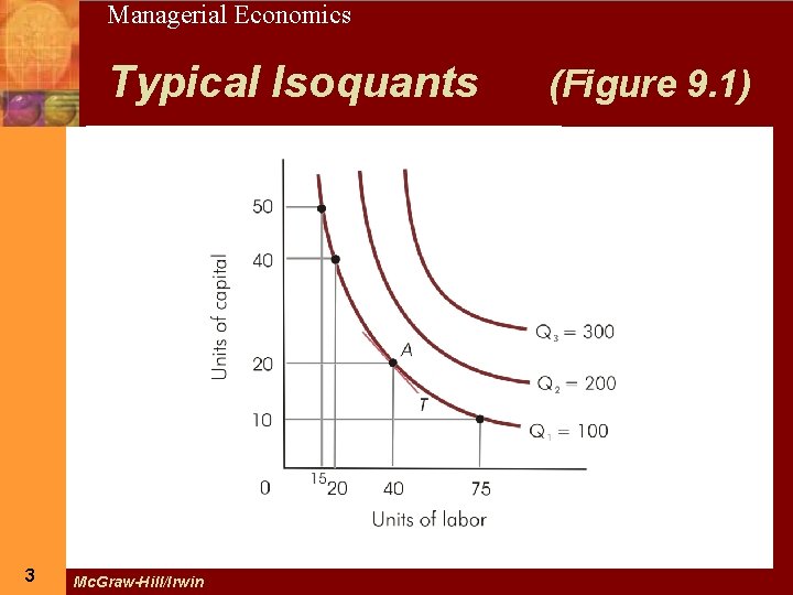
2 Managerial Economics Production Isoquants • In the long run, all inputs are variable & isoquants are used to study production decisions • An isoquant is a curve showing all possible input combinations capable of producing a given level of output • Isoquants are downward sloping; if greater amounts of labor are used, less capital is required to produce a given output 2 Mc. Graw-Hill/Irwin

3 Managerial Economics Typical Isoquants 3 Mc. Graw-Hill/Irwin (Figure 9. 1)

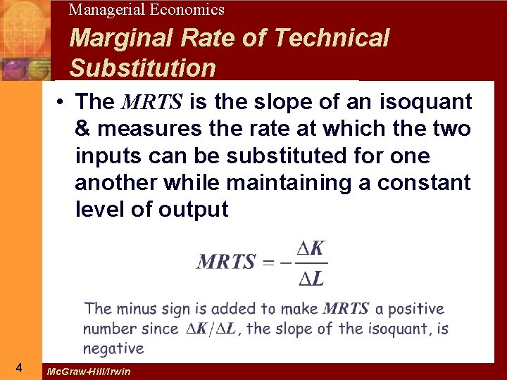
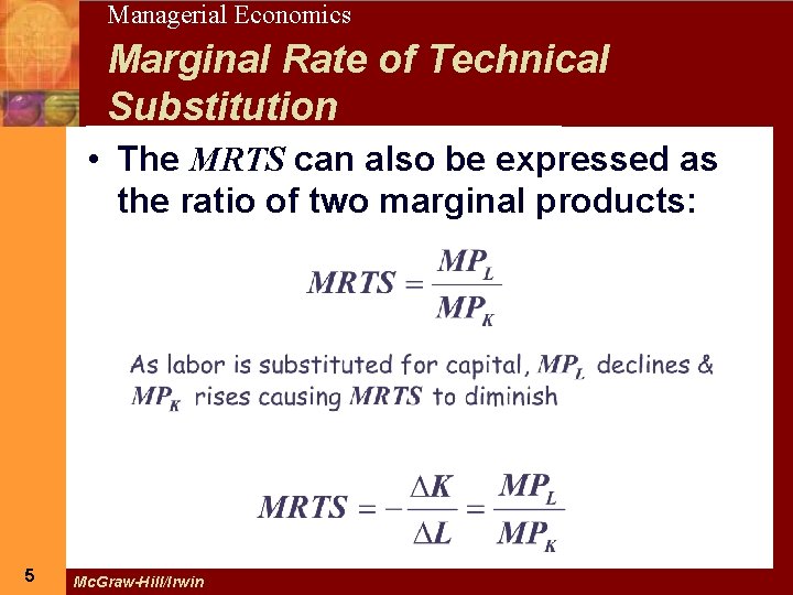
4 Managerial Economics Marginal Rate of Technical Substitution • The MRTS is the slope of an isoquant & measures the rate at which the two inputs can be substituted for one another while maintaining a constant level of output 4 Mc. Graw-Hill/Irwin

5 Managerial Economics Marginal Rate of Technical Substitution • The MRTS can also be expressed as the ratio of two marginal products: 5 Mc. Graw-Hill/Irwin

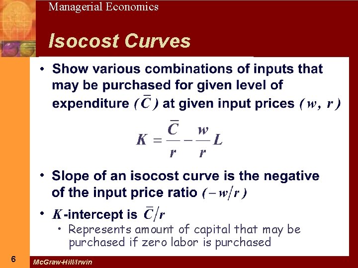
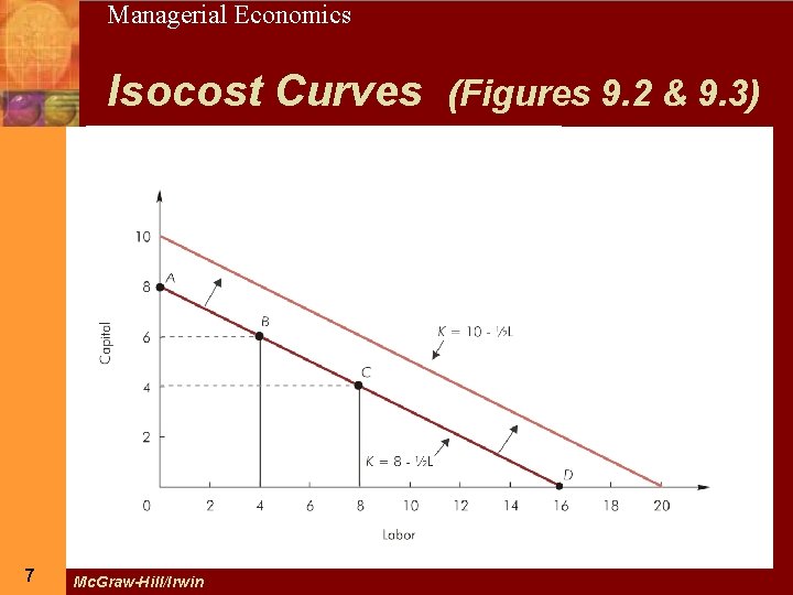
Managerial Economics 6 Isocost Curves • • • 6 • Represents amount of capital that may be purchased if zero labor is purchased Mc. Graw-Hill/Irwin

7 Managerial Economics Isocost Curves (Figures 9. 2 & 9. 3) 7 Mc. Graw-Hill/Irwin

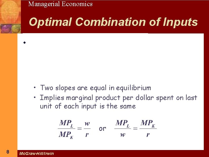
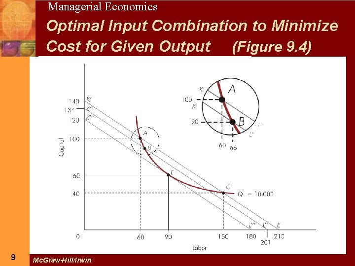
Managerial Economics 8 Optimal Combination of Inputs • • Two slopes are equal in equilibrium • Implies marginal product per dollar spent on last unit of each input is the same 8 Mc. Graw-Hill/Irwin

9 Managerial Economics Optimal Input Combination to Minimize Cost for Given Output (Figure 9. 4) 9 Mc. Graw-Hill/Irwin

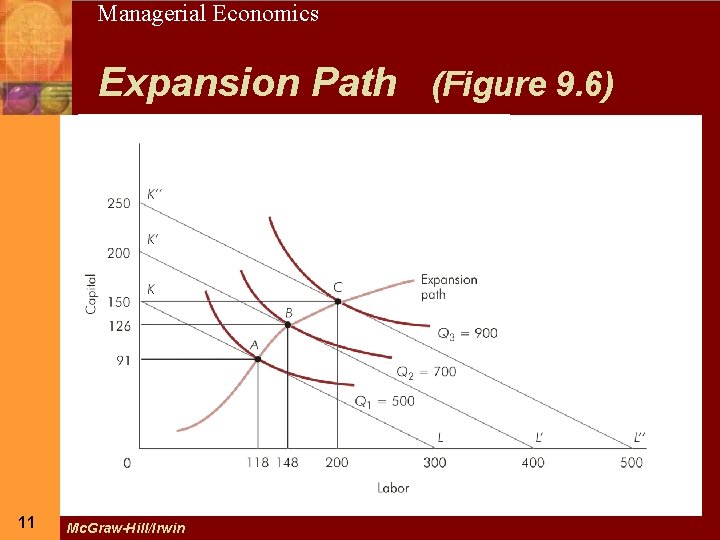
10 Managerial Economics Optimization & Cost • Expansion path gives the efficient (least-cost) input combinations for every level of output • Derived for a specific set of input prices • Along expansion path, input-price ratio is constant & equal to the marginal rate of technical substitution 10 Mc. Graw-Hill/Irwin

11 Managerial Economics Expansion Path (Figure 9. 6) 11 Mc. Graw-Hill/Irwin

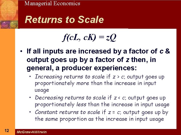
12 Managerial Economics Returns to Scale f(c. L, c. K) = z. Q • If all inputs are increased by a factor of c & output goes up by a factor of z then, in general, a producer experiences: • Increasing returns to scale if z > c; output goes up proportionately more than the increase in input usage • Decreasing returns to scale if z < c; output goes up proportionately less than the increase in input usage • Constant returns to scale if z = c; output goes up by the same proportion as the increase in input usage 12 Mc. Graw-Hill/Irwin

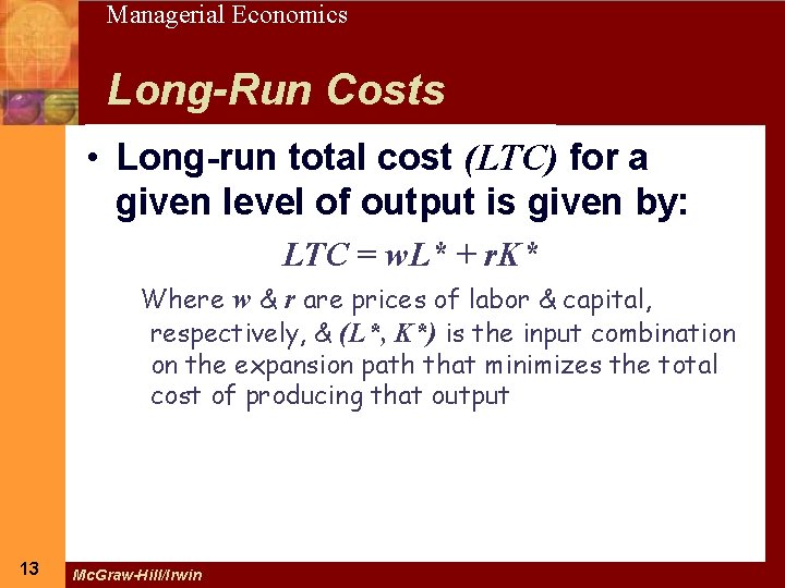
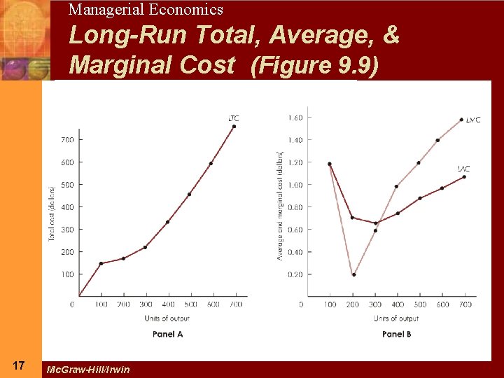
13 Managerial Economics Long-Run Costs • Long-run total cost (LTC) for a given level of output is given by: LTC = w. L* + r. K* Where w & r are prices of labor & capital, respectively, & (L*, K*) is the input combination on the expansion path that minimizes the total cost of producing that output 13 Mc. Graw-Hill/Irwin

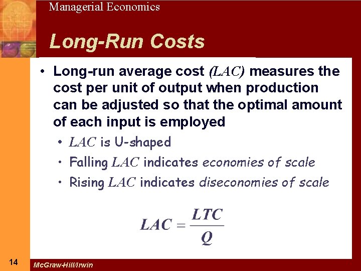
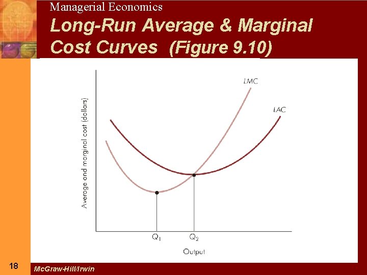
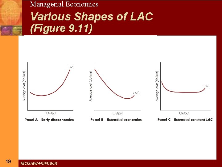
14 Managerial Economics Long-Run Costs • Long-run average cost (LAC) measures the cost per unit of output when production can be adjusted so that the optimal amount of each input is employed • LAC is U-shaped • Falling LAC indicates economies of scale • Rising LAC indicates diseconomies of scale 14 Mc. Graw-Hill/Irwin

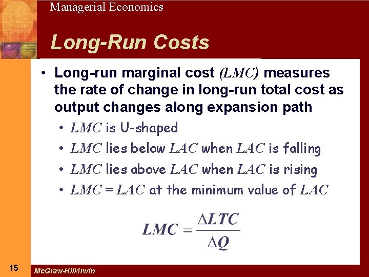
15 Managerial Economics Long-Run Costs • Long-run marginal cost (LMC) measures the rate of change in long-run total cost as output changes along expansion path • LMC is U-shaped • LMC lies below LAC when LAC is falling • LMC lies above LAC when LAC is rising • LMC = LAC at the minimum value of LAC 15 Mc. Graw-Hill/Irwin

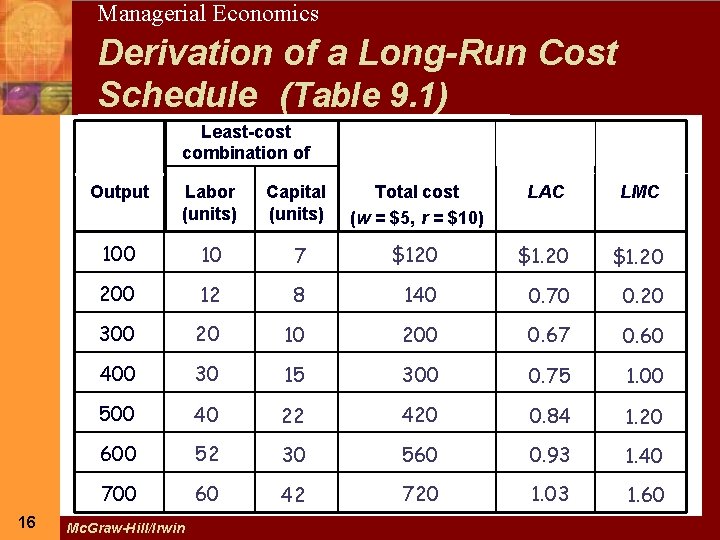
16 Managerial Economics Derivation of a Long-Run Cost Schedule (Table 9. 1) Least-cost combination of 16 Output Labor (units) Capital (units) Total cost (w = $5, r = $10) LAC LMC 100 10 7 $120 $1. 20 200 12 8 140 0. 70 0. 20 300 20 10 200 0. 67 0. 60 400 30 15 300 0. 75 1. 00 500 40 22 420 0. 84 1. 20 600 52 30 560 0. 93 1. 40 700 60 42 720 1. 03 1. 60 Mc. Graw-Hill/Irwin

17 17 Managerial Economics Long-Run Total, Average, & Marginal Cost (Figure 9. 9) Mc. Graw-Hill/Irwin

18 18 Managerial Economics Long-Run Average & Marginal Cost Curves (Figure 9. 10) Mc. Graw-Hill/Irwin

19 Managerial Economics Various Shapes of LAC (Figure 9. 11) 19 Mc. Graw-Hill/Irwin

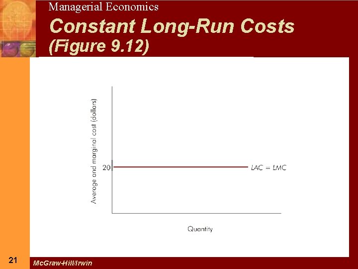
20 Managerial Economics Constant Long-Run Costs • When constant returns to scale occur over entire range of output • Firm experiences constant costs in the long run • LAC curve is flat & equal to LMC at all output levels 20 Mc. Graw-Hill/Irwin

21 Managerial Economics Constant Long-Run Costs (Figure 9. 12) 21 Mc. Graw-Hill/Irwin

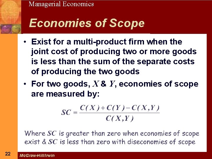
22 Managerial Economics Economies of Scope • Exist for a multi-product firm when the joint cost of producing two or more goods is less than the sum of the separate costs of producing the two goods • For two goods, X & Y, economies of scope are measured by: 22 Mc. Graw-Hill/Irwin

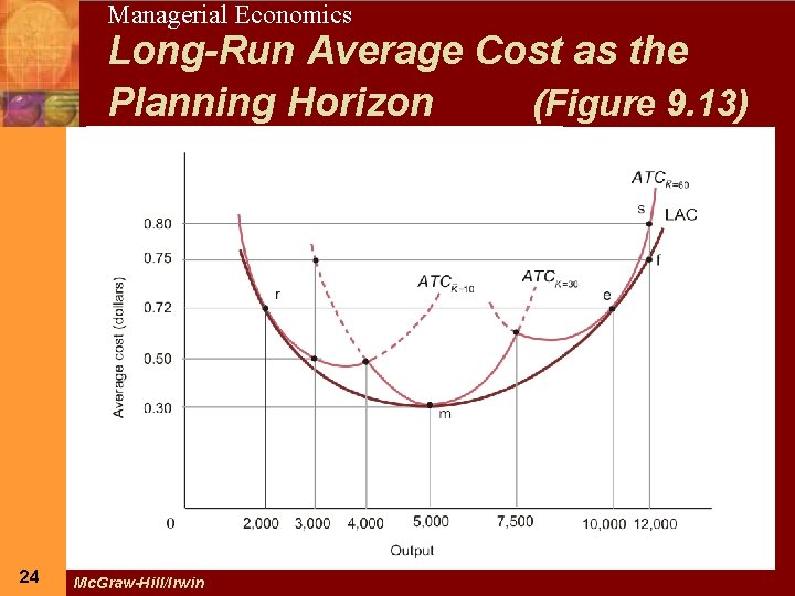
23 Managerial Economics Relations Between Short-Run & Long-Run Costs • LMC intersects LAC when the latter is at its minimum point • At each output where a particular ATC is tangent to LAC, the relevant SMC = LMC • For all ATC curves, point of tangency with LAC is at an output less (greater) than the output of minimum ATC if the tangency is at an output less (greater) than that associated with minimum LAC 23 Mc. Graw-Hill/Irwin

24 24 Managerial Economics Long-Run Average Cost as the Planning Horizon (Figure 9. 13) Mc. Graw-Hill/Irwin

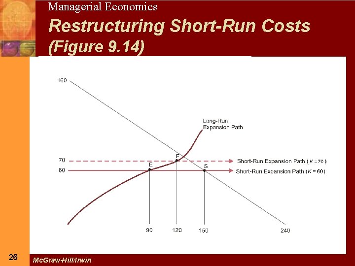
25 Managerial Economics Restructuring Short-Run Costs • Because managers have greatest flexibility to choose inputs in the long run, costs are lower in the long run than in the short run for all output levels except that for which the fixed input is at its optimal level • Short-run costs can be reduced by adjusting fixed inputs to their optimal long-run levels when the opportunity arises 25 Mc. Graw-Hill/Irwin

26 Managerial Economics Restructuring Short-Run Costs (Figure 9. 14) 26 Mc. Graw-Hill/Irwin