MANAGERIAL ECONOMICS ECON 5133 Lesson Thirteen DERIVATIVE SIGNALS

I. A marginal’s signaling capability A. A marginal gives the rate of change of

If TR = 700 Qx -. 01 Qx then 2 MR = 700 -.

TR = 700 Qx -. 01 Qx 2 TR ($M) When MR > 0,

D. Summary 1. Marginals signal rates of change of their “parent” 2. Graphically marginals

II. Derivatives are hierarchical Parent Function (TR; TC) Child (1 st derivative) (MR; MC)

A. Example: A 3 o polynomial Step 1: find its derivative Step 2: find

Step 3: Evaluate derivative near critical values X 1 1. 5 2 d. Y/d.

Step 4: sketch tangent pattern at points of evaluation and nearby Y Pattern for

Step 5: find inflection points (where the parent curve changes direction) at an inflection

Inflection Type 1: the parent curve stops increasing at a decreasing rate and starts

Inflection Type 2 a: the parent curve stops decreasing at an increasing rate and

Inflection Type 2 b: the parent curve stops increasing at an increasing rate and

Step 6: locating inflection points a. find the second derivative it’s a derivative of

b. find points where the second derivative is zero these are points where the

Step 7: reading marginal signals X d. Y/d. X d. Y 2/d. X 2

Step 8: summary of marginal signals if d. Y/d. X changes from + to

Step 9: sketch tangent pattern at points of evaluation and nearby + 0 Y

This is an actual computer plot of the original function

B. Example: another 3 o polynomial Step 1: find its derivative Step 2: find

Step 3: locate inflection points a. find second derivative b. find points where the

Step 4: Evaluate all near critical values of X X Q d. Q/d. X

Assignment 6 You are now ready to complete Assignment 6. Click on the Assignment

Slides: 28

Download presentation

MANAGERIAL ECONOMICS ECON 5133, Lesson Thirteen DERIVATIVE SIGNALS Marginals’ signaling function Graphical representations It’s a Family Affair Finding Extrema Copyright © 2005 by George A. Collier Jr.

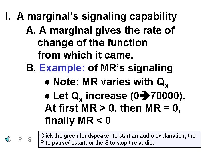
I. A marginal’s signaling capability A. A marginal gives the rate of change of the function from which it came. B. Example: of MR’s signaling Note: MR varies with Qx Let Qx increase (0 70000). At first MR > 0, then MR = 0, finally MR < 0 P S Click the green loudspeaker to start an audio explanation, the P to pause/restart, or the S to stop the audio.

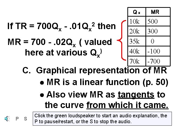
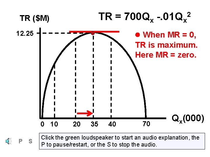
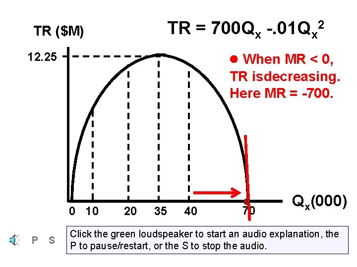
If TR = 700 Qx -. 01 Qx then 2 MR = 700 -. 02 Qx ( valued here at various Qx) Qx MR 10 k 20 k 35 k 40 k 70 k 500 300 0 -100 -700 C. Graphical representation of MR is a linear function (p. 50) Also view MR as tangents to the curve from which it came. P S Click the green loudspeaker to start an audio explanation, the P to pause/restart, or the S to stop the audio.

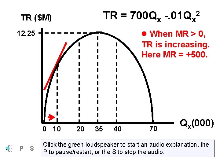
TR = 700 Qx -. 01 Qx 2 TR ($M) When MR > 0, 12. 25 TR is increasing. Here MR = +500. 0 10 P S 20 35 40 70 Qx(000) Click the green loudspeaker to start an audio explanation, the P to pause/restart, or the S to stop the audio.

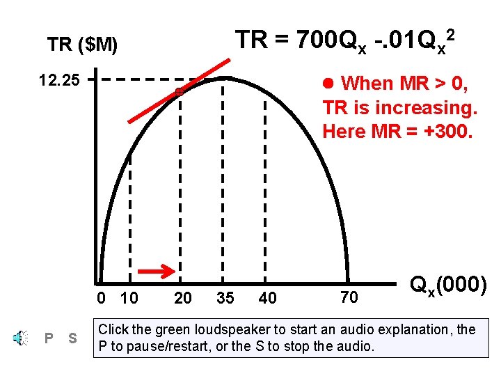
TR = 700 Qx -. 01 Qx 2 TR ($M) When MR > 0, 12. 25 TR is increasing. Here MR = +300. 0 10 P S 20 35 40 70 Qx(000) Click the green loudspeaker to start an audio explanation, the P to pause/restart, or the S to stop the audio.

TR = 700 Qx -. 01 Qx 2 TR ($M) When MR = 0, 12. 25 TR is maximum. Here MR = zero. 0 10 P S 20 35 40 70 Qx(000) Click the green loudspeaker to start an audio explanation, the P to pause/restart, or the S to stop the audio.

TR = 700 Qx -. 01 Qx 2 TR ($M) When MR < 0, 12. 25 TR is decreasing. Here MR = -100. 0 10 P S 20 35 40 70 Qx(000) Click the green loudspeaker to start an audio explanation, the P to pause/restart, or the S to stop the audio.

TR = 700 Qx -. 01 Qx 2 TR ($M) When MR < 0, 12. 25 TR isdecreasing. Here MR = -700. 0 10 P S 20 35 40 70 Qx(000) Click the green loudspeaker to start an audio explanation, the P to pause/restart, or the S to stop the audio.

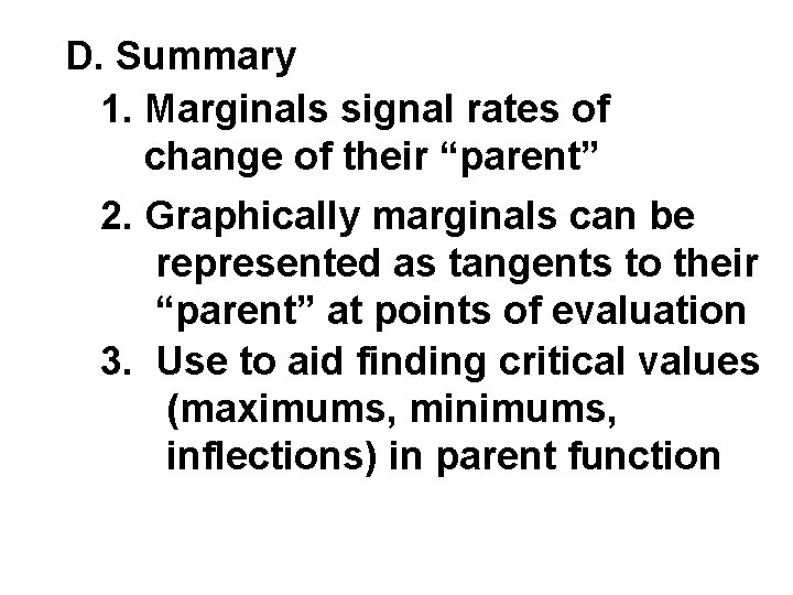
D. Summary 1. Marginals signal rates of change of their “parent” 2. Graphically marginals can be represented as tangents to their “parent” at points of evaluation 3. Use to aid finding critical values (maximums, minimums, inflections) in parent function

II. Derivatives are hierarchical Parent Function (TR; TC) Child (1 st derivative) (MR; MC) Grandchild (2 nd derivative) 3 rd derivative, etc. P S Click the green loudspeaker to start an audio explanation, the P to pause/restart, or the S to stop the audio.

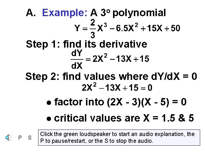
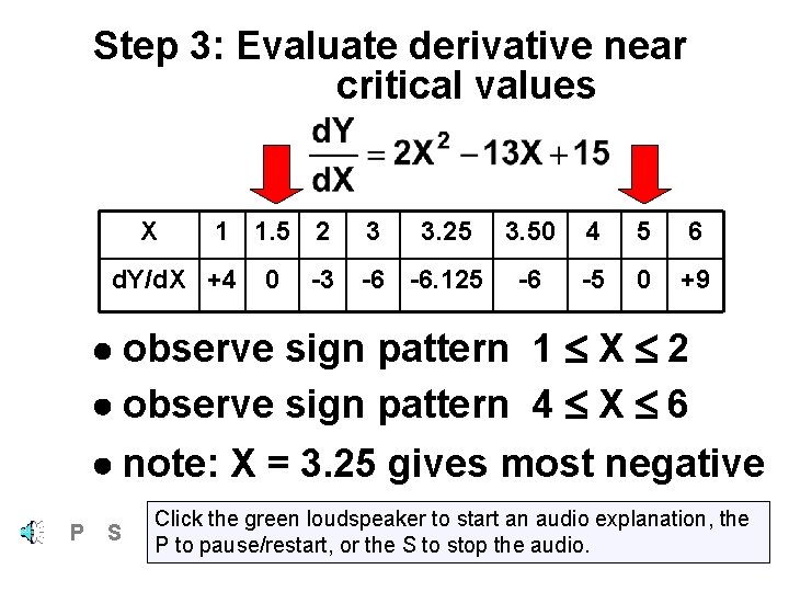
A. Example: A 3 o polynomial Step 1: find its derivative Step 2: find values where d. Y/d. X = 0 factor into (2 X - 3)(X - 5) = 0 critical values are X = 1. 5 & 5 P S Click the green loudspeaker to start an audio explanation, the P to pause/restart, or the S to stop the audio.

Step 3: Evaluate derivative near critical values X 1 1. 5 2 d. Y/d. X +4 0 -3 3 3. 25 -6 -6. 125 3. 50 4 5 6 -6 -5 0 +9 observe sign pattern 1 X 2 observe sign pattern 4 X 6 note: X = 3. 25 gives most negative P S Click the green loudspeaker to start an audio explanation, the P to pause/restart, or the S to stop the audio.

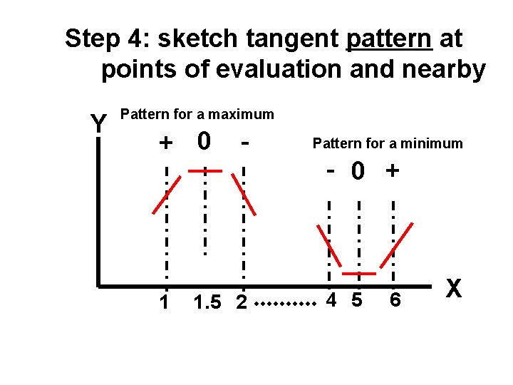
Step 4: sketch tangent pattern at points of evaluation and nearby Y Pattern for a maximum + 0 1 - 1. 5 2 Pattern for a minimum - 0 + 4 5 6 X

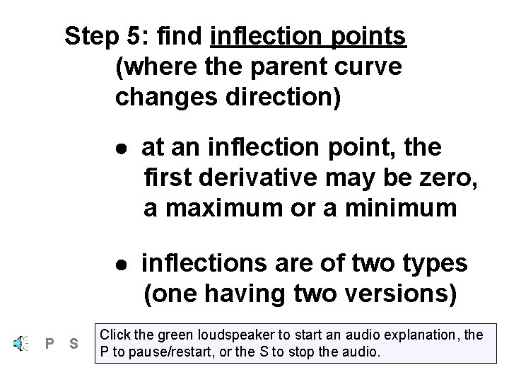
Step 5: find inflection points (where the parent curve changes direction) at an inflection point, the first derivative may be zero, a maximum or a minimum inflections are of two types (one having two versions) P S Click the green loudspeaker to start an audio explanation, the P to pause/restart, or the S to stop the audio.

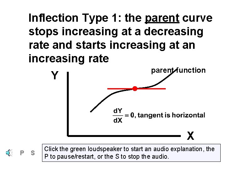
Inflection Type 1: the parent curve stops increasing at a decreasing rate and starts increasing at an increasing rate parent function Y X P S Click the green loudspeaker to start an audio explanation, the P to pause/restart, or the S to stop the audio.

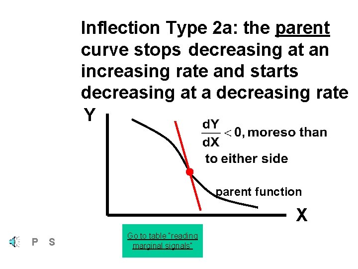
Inflection Type 2 a: the parent curve stops decreasing at an increasing rate and starts decreasing at a decreasing rate Y parent function X P S Go to table “reading marginal signals”

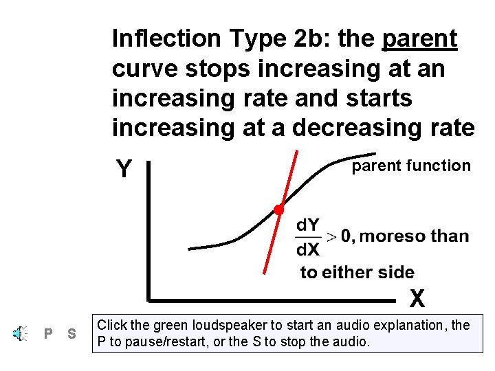
Inflection Type 2 b: the parent curve stops increasing at an increasing rate and starts increasing at a decreasing rate Y parent function X P S Click the green loudspeaker to start an audio explanation, the P to pause/restart, or the S to stop the audio.

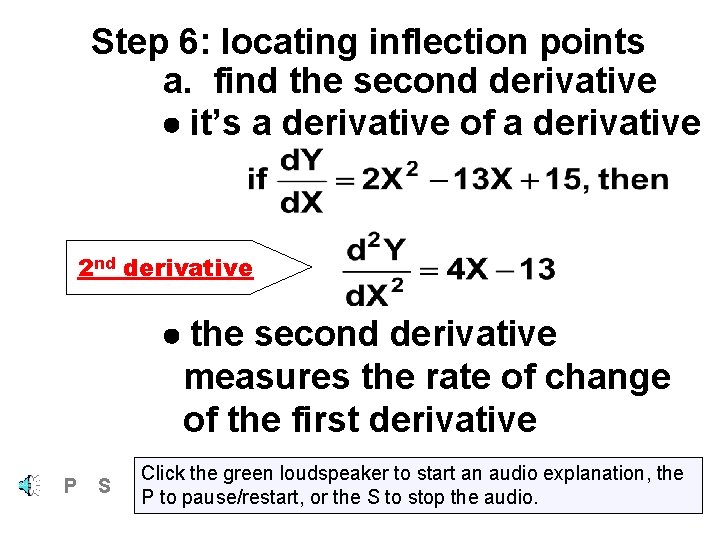
Step 6: locating inflection points a. find the second derivative it’s a derivative of a derivative 2 nd derivative the second derivative measures the rate of change of the first derivative P S Click the green loudspeaker to start an audio explanation, the P to pause/restart, or the S to stop the audio.

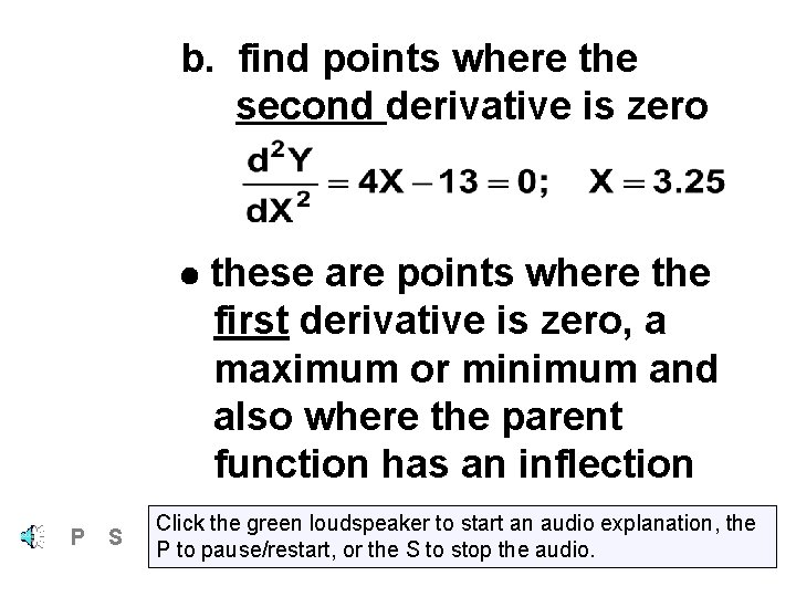
b. find points where the second derivative is zero these are points where the first derivative is zero, a maximum or minimum and also where the parent function has an inflection P S Click the green loudspeaker to start an audio explanation, the P to pause/restart, or the S to stop the audio.

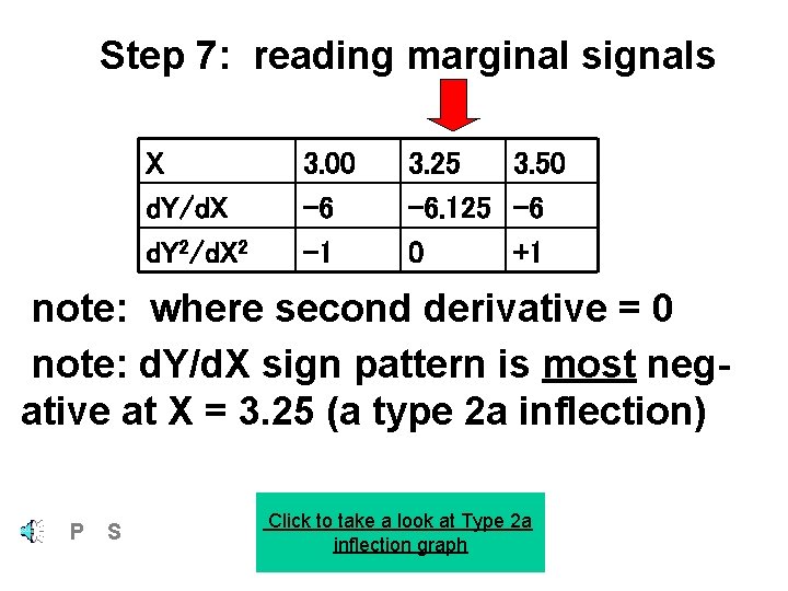
Step 7: reading marginal signals X d. Y/d. X d. Y 2/d. X 2 3. 00 -6 -1 3. 25 3. 50 -6. 125 -6 0 +1 note: where second derivative = 0 note: d. Y/d. X sign pattern is most negative at X = 3. 25 (a type 2 a inflection) P S Click to take a look at Type 2 a inflection graph

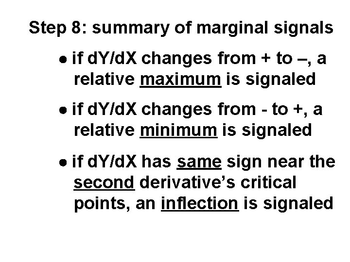
Step 8: summary of marginal signals if d. Y/d. X changes from + to –, a relative maximum is signaled if d. Y/d. X changes from - to +, a relative minimum is signaled if d. Y/d. X has same sign near the second derivative’s critical points, an inflection is signaled

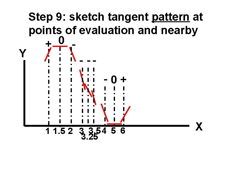
Step 9: sketch tangent pattern at points of evaluation and nearby + 0 Y - --0+ 1 1. 5 2 3 3. 5 4 5 6 3. 25 X

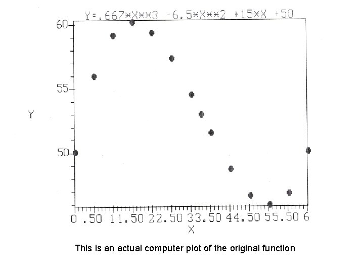
This is an actual computer plot of the original function

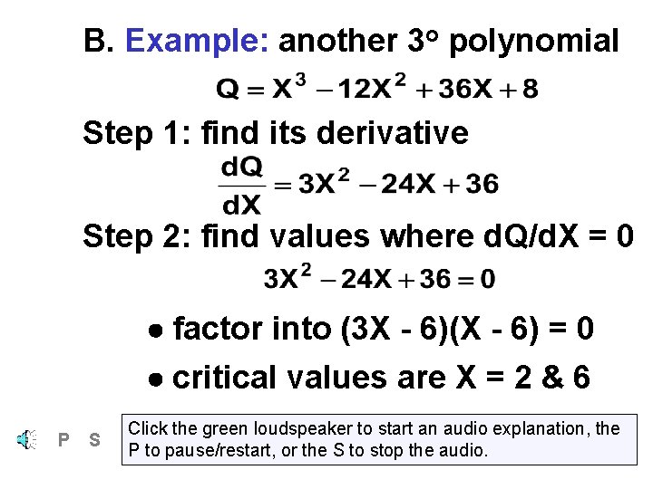
B. Example: another 3 o polynomial Step 1: find its derivative Step 2: find values where d. Q/d. X = 0 factor into (3 X - 6)(X - 6) = 0 critical values are X = 2 & 6 P S Click the green loudspeaker to start an audio explanation, the P to pause/restart, or the S to stop the audio.

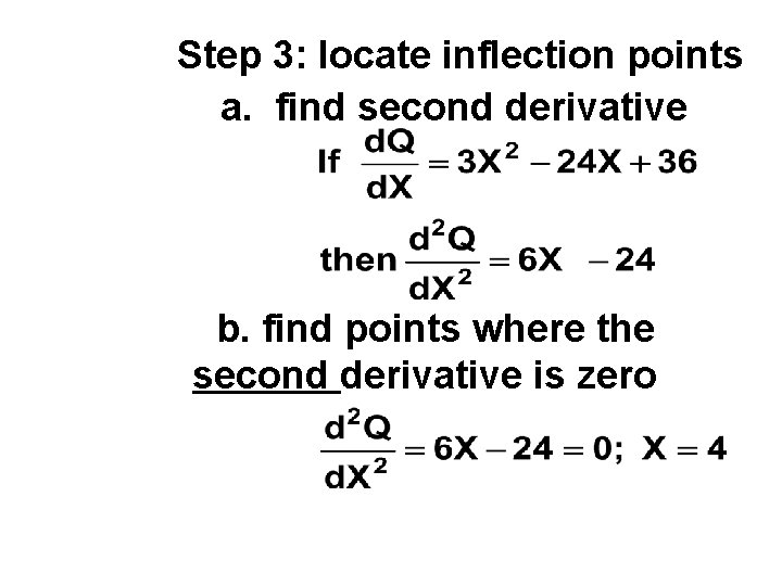
Step 3: locate inflection points a. find second derivative b. find points where the second derivative is zero

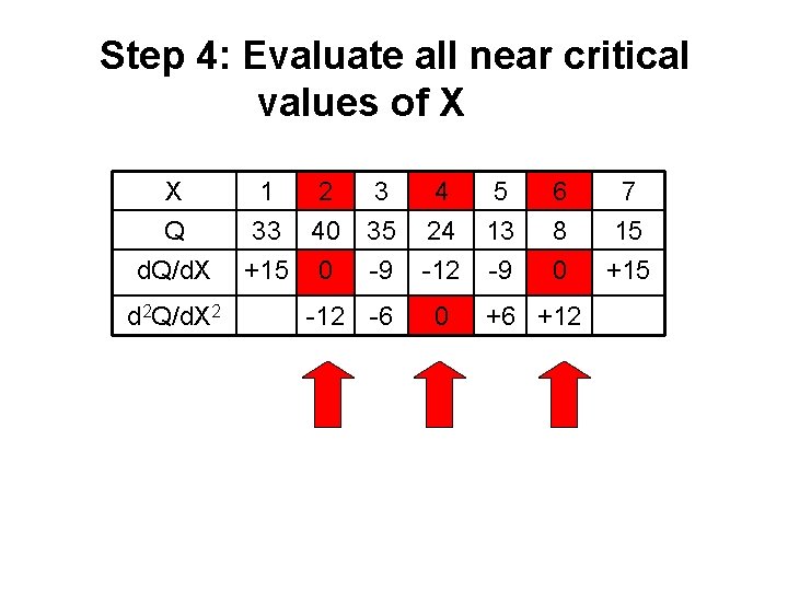
Step 4: Evaluate all near critical values of X X Q d. Q/d. X d 2 Q/d. X 2 1 2 33 40 +15 0 3 4 5 35 24 13 -9 -12 -6 0 6 8 0 +6 +12 7 15 +15

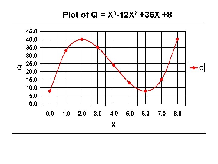
Plot of Q = X 3 -12 X 2 +36 X +8

Assignment 6 You are now ready to complete Assignment 6. Click on the Assignment Selector link, complete the form that appears, and submit it. You should receive an email at the address you entered into the form with your assignment number for the assignment. The assignment files are inside the Assignment 6 folder. You will find your version beside the number you were assigned. This is your personal exercise. Each is a Word™ document. Download your exercise and use Excel™ or another method to calculate the critical points of the function. Also notice the bonus opportunity that is a part of each exercise. Your completed assignment must be submitted by uploading it in Blackboard™. Be sure to follow the instructions posted in the Assignment 6 folder for submitting your assignment.