Managerial Economics Business Strategy Chapter 8 Managing in

Managerial Economics & Business Strategy Chapter 8 Managing in Competitive, Monopolistic, and Monopolistically Competitive Markets Mc. Graw-Hill/Irwin Michael R. Baye, Managerial Economics and Business Strategy Copyright © 2008 by the Mc. Graw-Hill Companies, Inc. All rights reserved.

Overview I. Perfect Competition • Characteristics and profit outlook. • Effect of new entrants. II. Monopolies • Sources of monopoly power. • Maximizing monopoly profits. • Pros and cons. III. Monopolistic Competition • Profit maximization. • Long run equilibrium. 8 -2

8 -3 Perfect Competition Environment • Many buyers and sellers. • Homogeneous (identical) product. • Perfect information on both sides of market. • No transaction costs. • Free entry and exit.

8 -4 Key Implications • Firms are “price takers” (P = MR). • In the short-run, firms may earn profits or losses. • Entry and exit forces long-run profits to zero.

8 -5 Unrealistic? Why Learn? • Many small businesses are “price-takers, ” and decision rules for such firms are similar to those of perfectly competitive firms. • It is a useful benchmark. • Explains why governments oppose monopolies. • Illuminates the “danger” to managers of competitive environments. • Importance of product differentiation. • Sustainable advantage.

8 -6 Managing a Perfectly Competitive Firm (or Price-Taking Business)

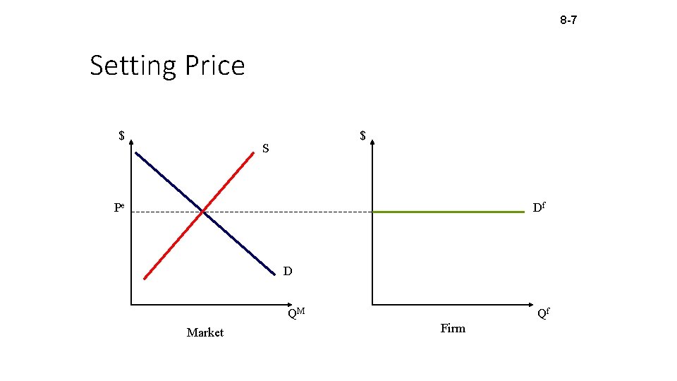
8 -7 Setting Price $ $ S Pe Df D QM Market Qf Firm

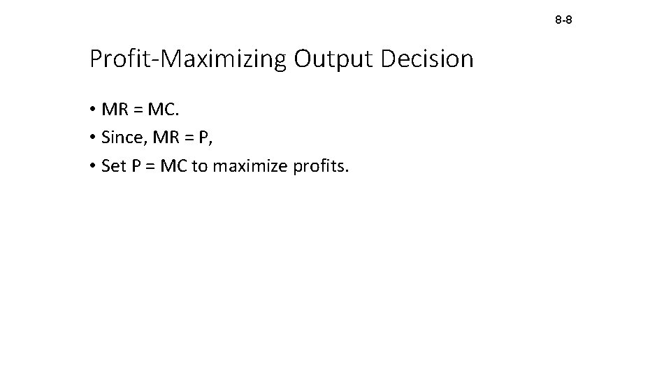
8 -8 Profit-Maximizing Output Decision • MR = MC. • Since, MR = P, • Set P = MC to maximize profits.

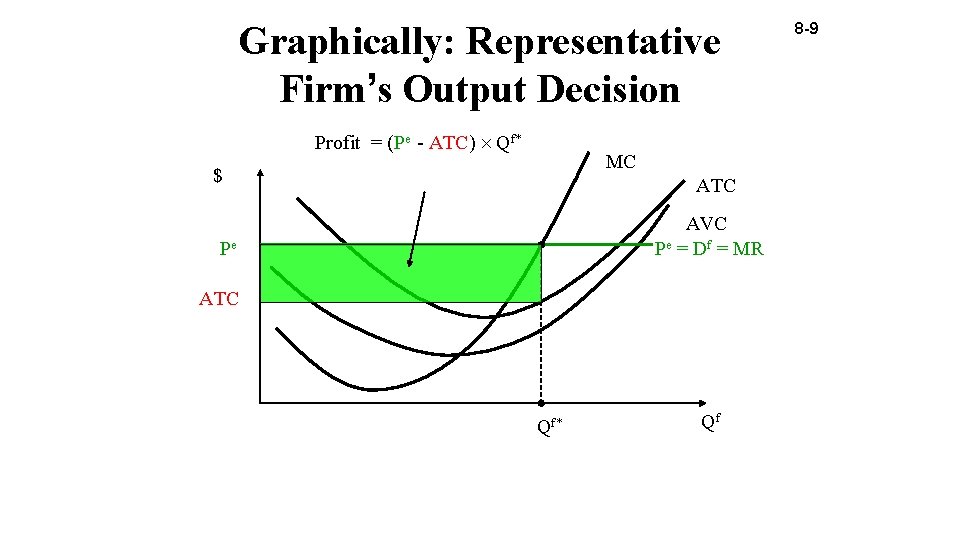
Graphically: Representative Firm’s Output Decision Profit = (Pe - ATC) Qf* MC $ ATC AVC Pe = Df = MR Pe ATC Qf* Qf 8 -9

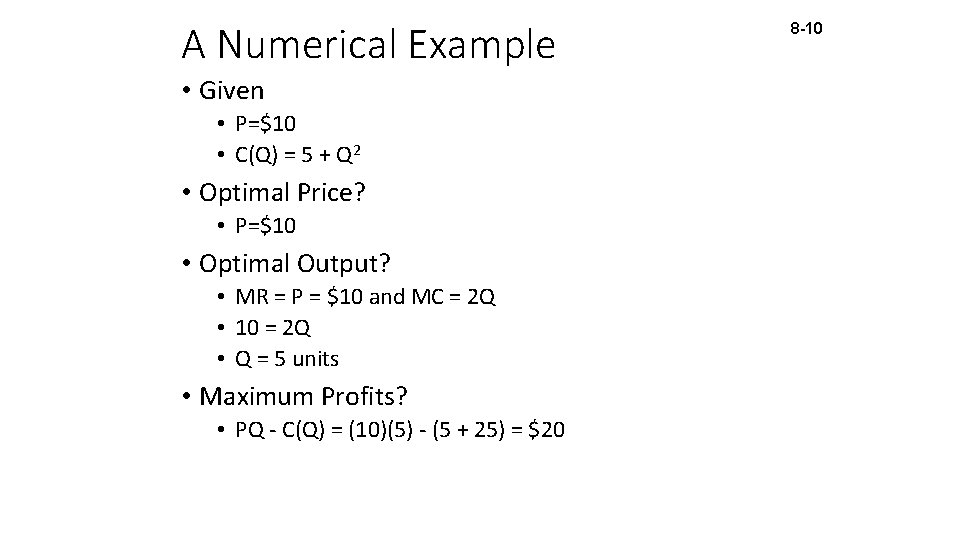
A Numerical Example • Given • P=$10 • C(Q) = 5 + Q 2 • Optimal Price? • P=$10 • Optimal Output? • MR = P = $10 and MC = 2 Q • 10 = 2 Q • Q = 5 units • Maximum Profits? • PQ - C(Q) = (10)(5) - (5 + 25) = $20 8 -10

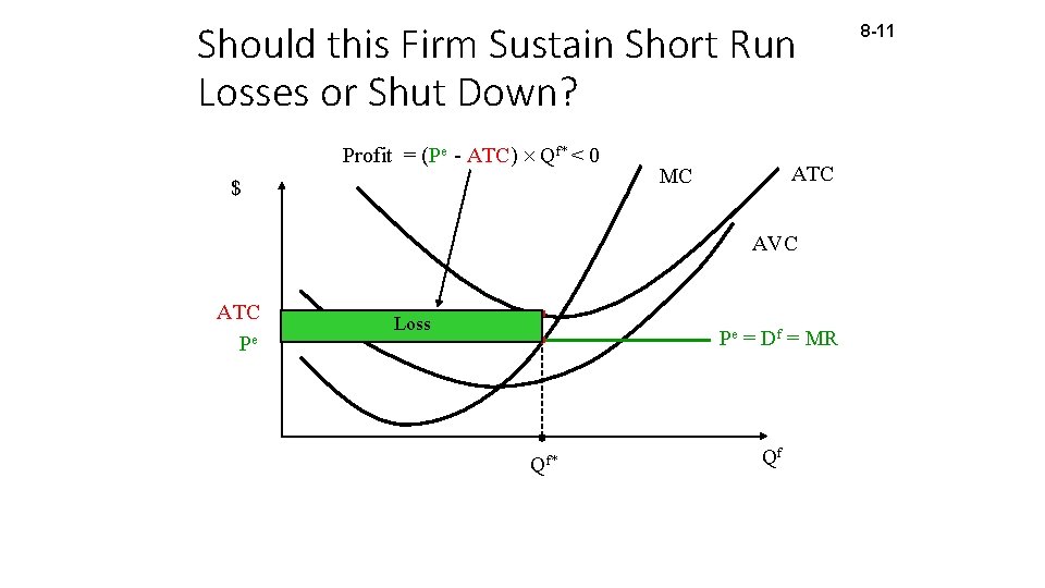
Should this Firm Sustain Short Run Losses or Shut Down? Profit = (Pe - ATC) Qf* < 0 $ ATC MC AVC ATC Pe Loss Pe = Df = MR Qf* Qf 8 -11

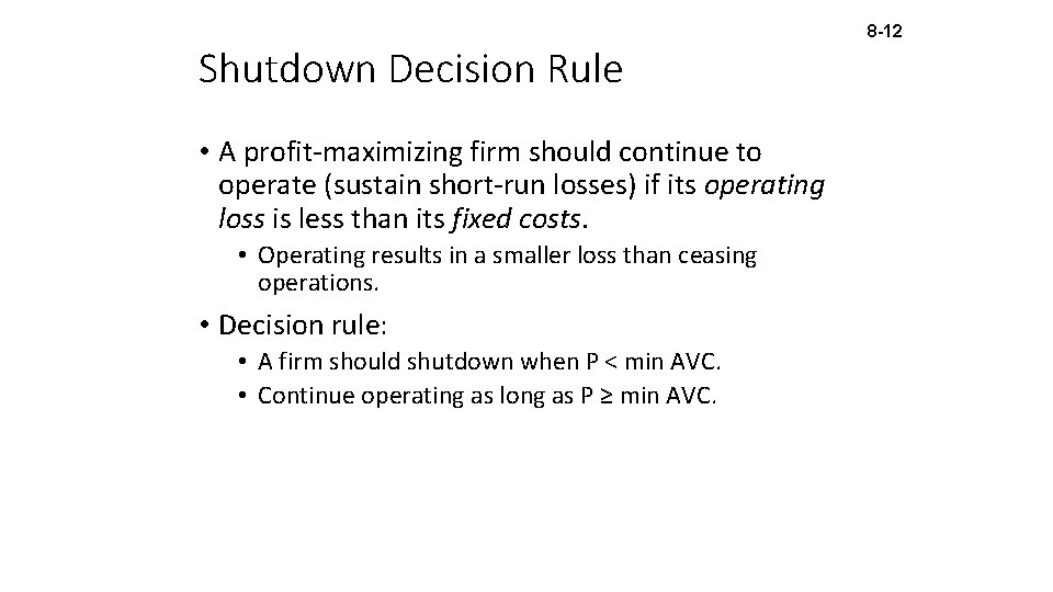
Shutdown Decision Rule • A profit-maximizing firm should continue to operate (sustain short-run losses) if its operating loss is less than its fixed costs. • Operating results in a smaller loss than ceasing operations. • Decision rule: • A firm should shutdown when P < min AVC. • Continue operating as long as P ≥ min AVC. 8 -12

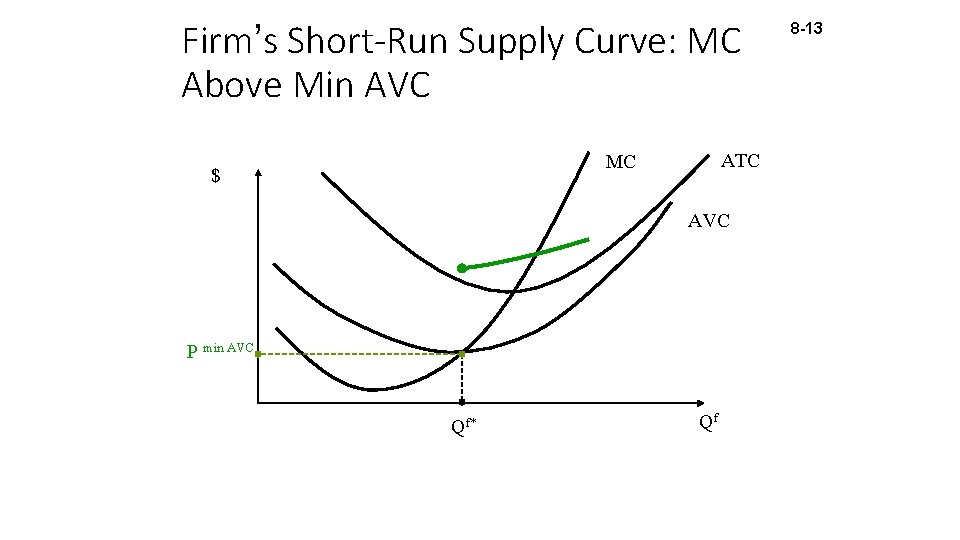
Firm’s Short-Run Supply Curve: MC Above Min AVC ATC MC $ AVC P min AVC Qf* Qf 8 -13

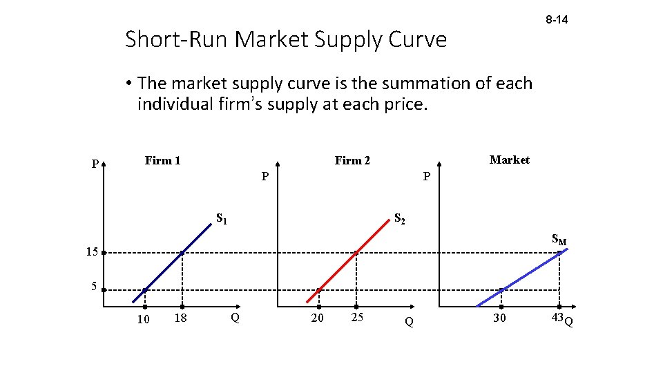
8 -14 Short-Run Market Supply Curve • The market supply curve is the summation of each individual firm’s supply at each price. P Firm 1 Market Firm 2 P P S 1 S 2 SM 15 5 10 18 Q 20 25 Q 30 43 Q

8 -15 Long Run Adjustments? • If firms are price takers but there are barriers to entry, profits will persist. • If the industry is perfectly competitive, firms are not only price takers but there is free entry. • Other “greedy capitalists” enter the market.

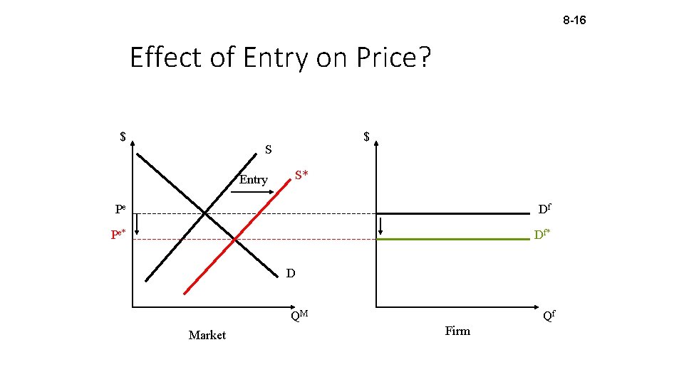
8 -16 Effect of Entry on Price? $ $ S Entry S* Pe Df Pe* Df* D QM Market Qf Firm

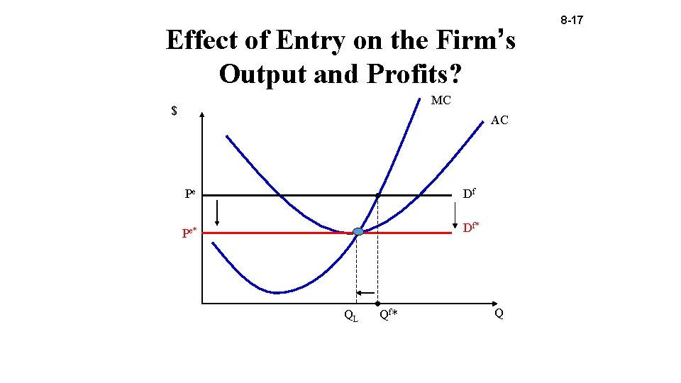
Effect of Entry on the Firm’s Output and Profits? MC $ AC Pe Df Pe* Df* QL Qf * Q 8 -17

8 -18 Summary of Logic • Short run profits leads to entry. • Entry increases market supply, drives down the market price, increases the market quantity. • Demand for individual firm’s product shifts down. • Firm reduces output to maximize profit. • Long run profits are zero.

8 -19 Features of Long Run Competitive Equilibrium • P = MC • Socially efficient output. • P = minimum AC • Efficient plant size. • Zero profits • Firms are earning just enough to offset their opportunity cost.

8 -20 Monopoly Environment • Single firm serves the “relevant market. ” • Most monopolies are “local” monopolies. • The demand for the firm’s product is the market demand curve. • Firm has control over price. • But the price charged affects the quantity demanded of the monopolist’s product.

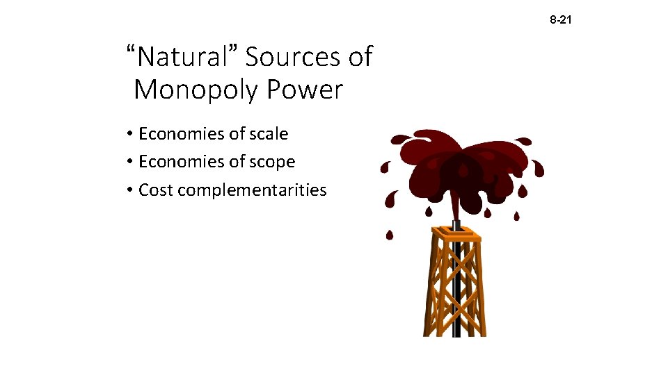
8 -21 “Natural” Sources of Monopoly Power • Economies of scale • Economies of scope • Cost complementarities

8 -22 “Created” Sources of Monopoly Power • Patents and other legal barriers (like licenses) • Tying contracts • Exclusive contracts • Collusion Contract. . . I. III.

8 -23 Managing a Monopoly • Market power permits you to price above MC • Is the sky the limit? • No. How much you sell depends on the price you set!

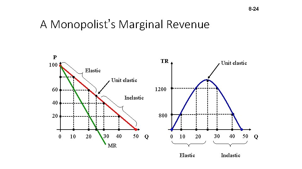
8 -24 A Monopolist’s Marginal Revenue P 100 TR Unit elastic Elastic Unit elastic 1200 60 Inelastic 40 800 20 0 10 20 30 40 50 Q 0 10 20 30 40 MR Elastic Inelastic 50 Q

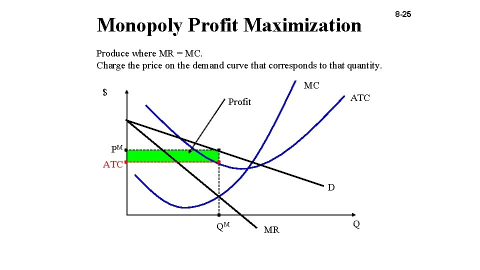
Monopoly Profit Maximization Produce where MR = MC. Charge the price on the demand curve that corresponds to that quantity. MC $ ATC Profit PM ATC D QM MR Q 8 -25

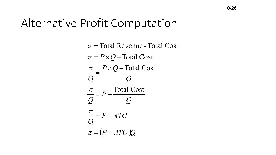
8 -26 Alternative Profit Computation

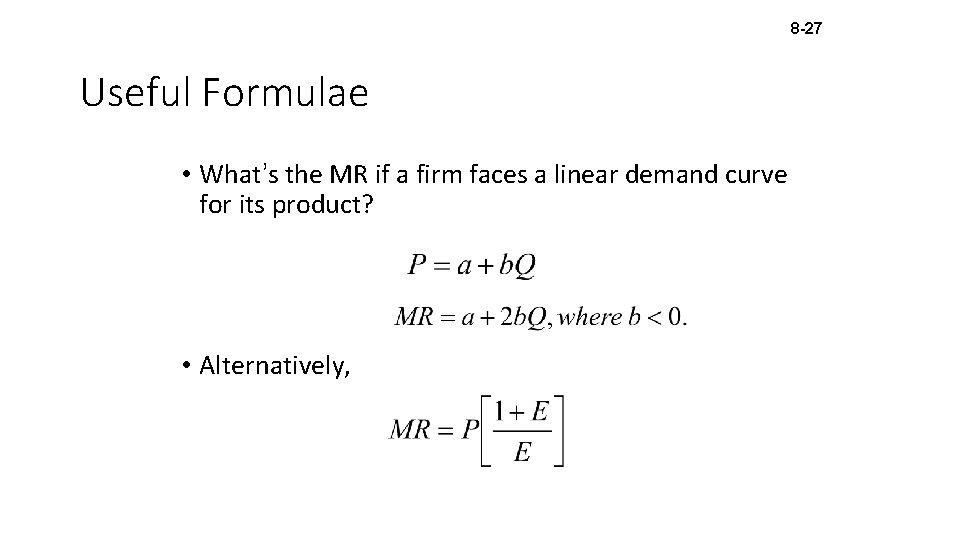
8 -27 Useful Formulae • What’s the MR if a firm faces a linear demand curve for its product? • Alternatively,

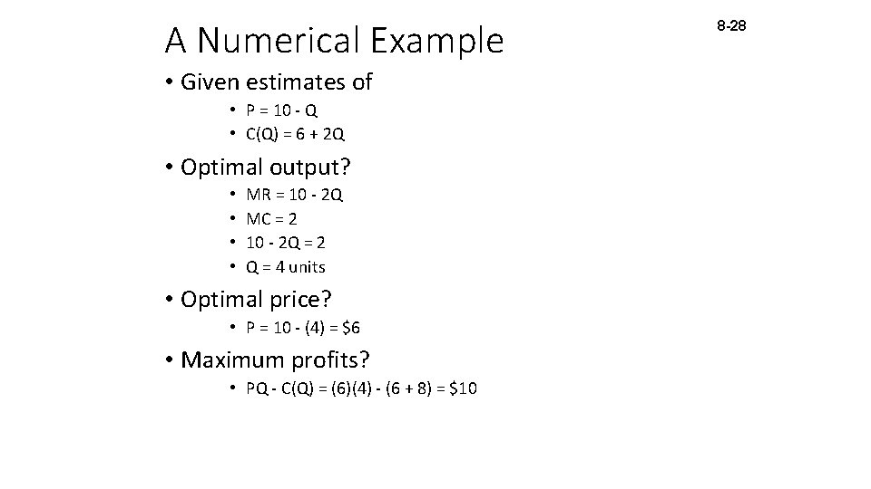
A Numerical Example • Given estimates of • P = 10 - Q • C(Q) = 6 + 2 Q • Optimal output? • • MR = 10 - 2 Q MC = 2 10 - 2 Q = 2 Q = 4 units • Optimal price? • P = 10 - (4) = $6 • Maximum profits? • PQ - C(Q) = (6)(4) - (6 + 8) = $10 8 -28

8 -29 Long Run Adjustments? • None, unless the source of monopoly power is eliminated.

8 -30 Why Government Dislikes Monopoly? • P > MC • Too little output, at too high a price. • Deadweight loss of monopoly.

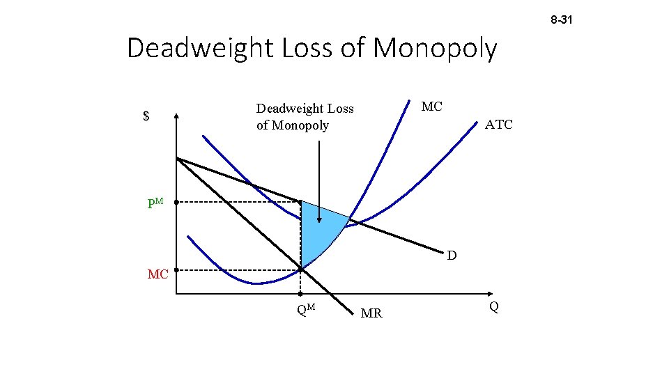
8 -31 Deadweight Loss of Monopoly $ MC Deadweight Loss of Monopoly ATC PM D MC QM MR Q

8 -32 Arguments for Monopoly • The beneficial effects of economies of scale, economies of scope, and cost complementarities on price and output may outweigh the negative effects of market power. • Encourages innovation.

8 -33 Monopolistic Competition: Environment and Implications • Numerous buyers and sellers • Differentiated products • Implication: Since products are differentiated, each firm faces a downward sloping demand curve. • Consumers view differentiated products as close substitutes: there exists some willingness to substitute. • Free entry and exit • Implication: Firms will earn zero profits in the long run.

Managing a Monopolistically Competitive Firm • Like a monopoly, monopolistically competitive firms • have market power that permits pricing above marginal cost. • level of sales depends on the price it sets. • But … • The presence of other brands in the market makes the demand for your brand more elastic than if you were a monopolist. • Free entry and exit impacts profitability. • Therefore, monopolistically competitive firms have limited market power. 8 -34

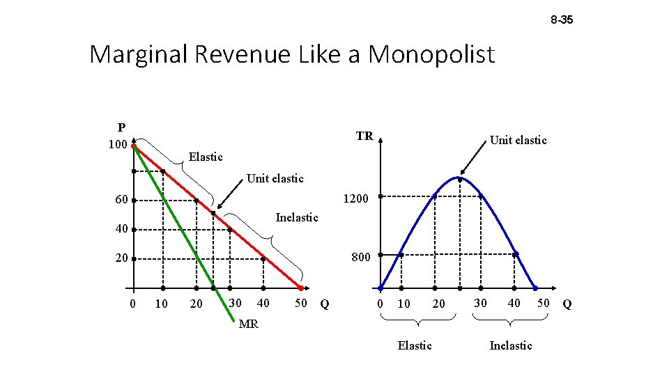
8 -35 Marginal Revenue Like a Monopolist P 100 TR Unit elastic Elastic Unit elastic 1200 60 Inelastic 40 800 20 0 10 20 30 40 50 Q 0 10 20 30 40 MR Elastic Inelastic 50 Q

8 -36 Monopolistic Competition: Profit Maximization • Maximize profits like a monopolist • Produce output where MR = MC. • Charge the price on the demand curve that corresponds to that quantity.

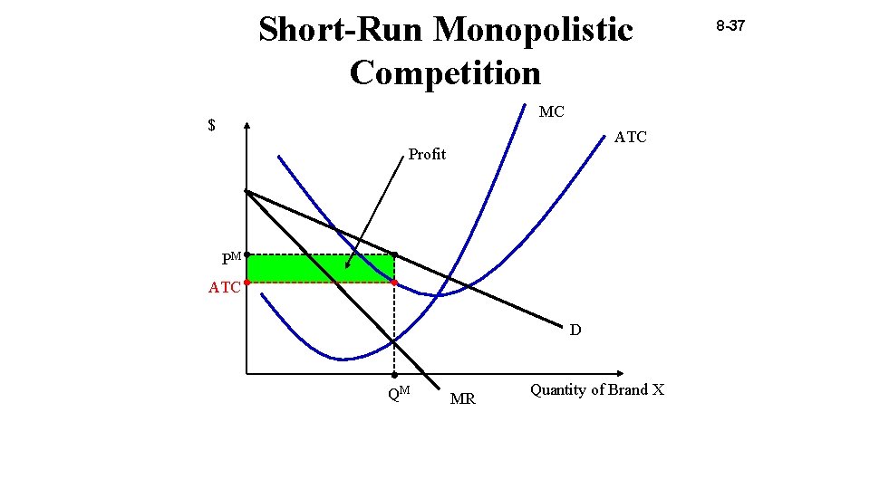
Short-Run Monopolistic Competition MC $ ATC Profit PM ATC D QM MR Quantity of Brand X 8 -37

8 -38 Long Run Adjustments? • If the industry is truly monopolistically competitive, there is free entry. • In this case other “greedy capitalists” enter, and their new brands steal market share. • This reduces the demand for your product until profits are ultimately zero.

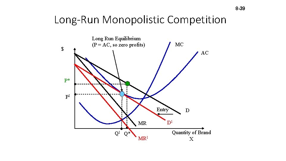
8 -39 Long-Run Monopolistic Competition Long Run Equilibrium (P = AC, so zero profits) $ MC AC P* P 1 Entry MR Q 1 Q* MR 1 D D 1 Quantity of Brand X

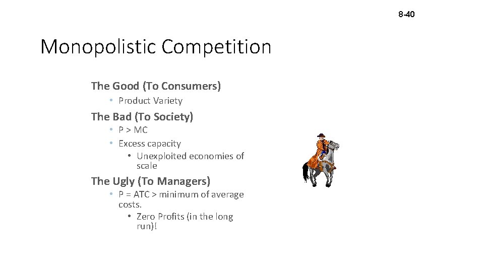
8 -40 Monopolistic Competition The Good (To Consumers) • Product Variety The Bad (To Society) • P > MC • Excess capacity • Unexploited economies of scale The Ugly (To Managers) • P = ATC > minimum of average costs. • Zero Profits (in the long run)!

Maximizing Profits: A Synthesizing Example 8 -41 • C(Q) = 125 + 4 Q 2 • Determine the profit-maximizing output and price, and discuss its implications, if • You are a price taker and other firms charge $40 per unit; • You are a monopolist and the inverse demand for your product is P = 100 - Q; • You are a monopolistically competitive firm and the inverse demand for your brand is P = 100 – Q.

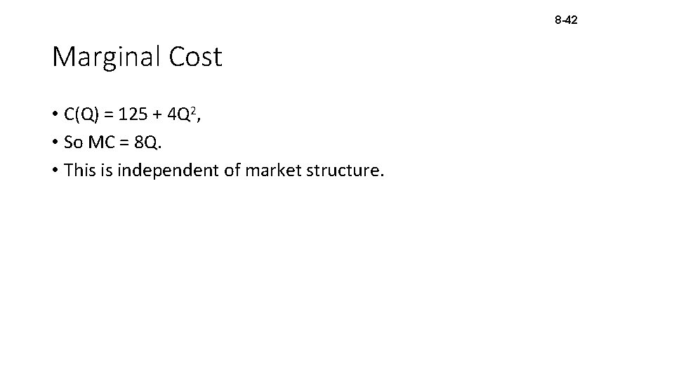
8 -42 Marginal Cost • C(Q) = 125 + 4 Q 2, • So MC = 8 Q. • This is independent of market structure.

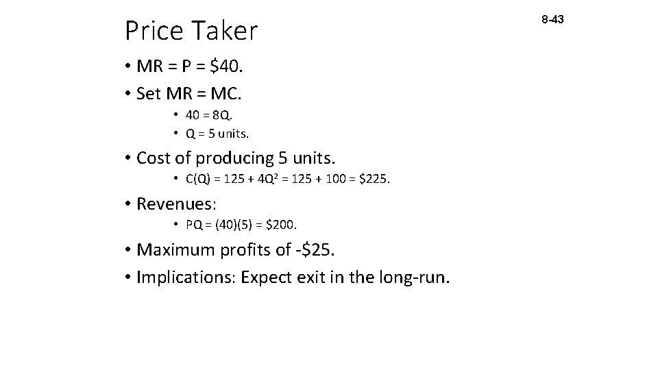
Price Taker • MR = P = $40. • Set MR = MC. • 40 = 8 Q. • Q = 5 units. • Cost of producing 5 units. • C(Q) = 125 + 4 Q 2 = 125 + 100 = $225. • Revenues: • PQ = (40)(5) = $200. • Maximum profits of -$25. • Implications: Expect exit in the long-run. 8 -43

Monopoly/Monopolistic Competition 8 -44 • MR = 100 - 2 Q (since P = 100 - Q). • Set MR = MC, or 100 - 2 Q = 8 Q. • Optimal output: Q = 10. • Optimal price: P = 100 - (10) = $90. • Maximal profits: • PQ - C(Q) = (90)(10) -(125 + 4(100)) = $375. • Implications • Monopolist will not face entry (unless patent or other entry barriers are eliminated). • Monopolistically competitive firm should expect other firms to clone, so profits will decline over time.

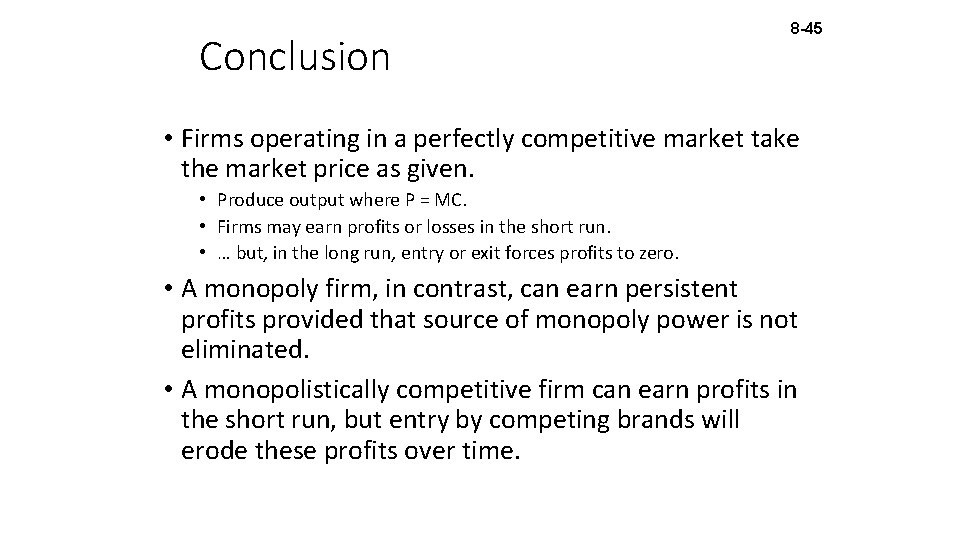
Conclusion 8 -45 • Firms operating in a perfectly competitive market take the market price as given. • Produce output where P = MC. • Firms may earn profits or losses in the short run. • … but, in the long run, entry or exit forces profits to zero. • A monopoly firm, in contrast, can earn persistent profits provided that source of monopoly power is not eliminated. • A monopolistically competitive firm can earn profits in the short run, but entry by competing brands will erode these profits over time.

Managerial Economics & Business Strategy Chapter 9 Basic Oligopoly Models Mc. Graw-Hill/Irwin Michael R. Baye, Managerial Economics and Business Strategy Copyright © 2008 by the Mc. Graw-Hill Companies, Inc. All rights reserved.

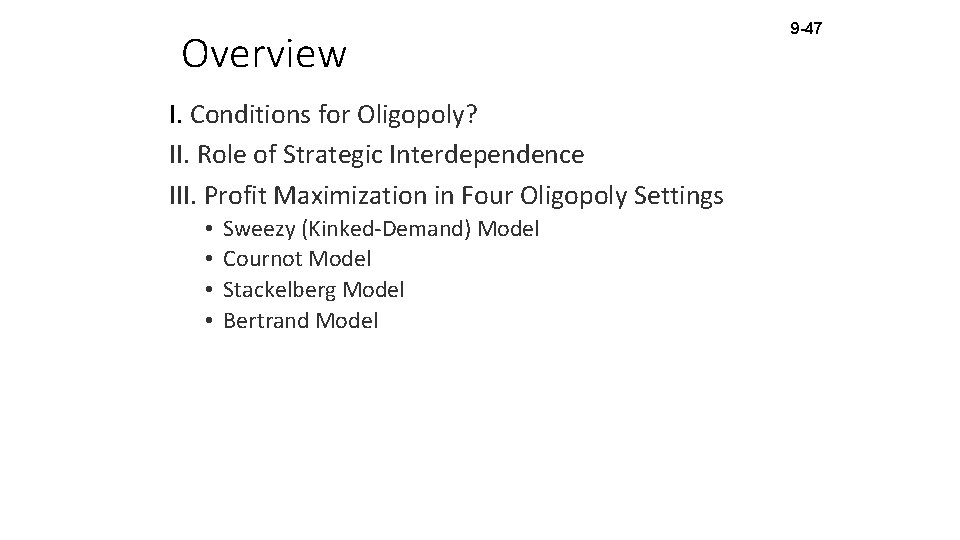
Overview I. Conditions for Oligopoly? II. Role of Strategic Interdependence III. Profit Maximization in Four Oligopoly Settings • • Sweezy (Kinked-Demand) Model Cournot Model Stackelberg Model Bertrand Model 9 -47

9 -48 Oligopoly Environment • Relatively few firms, usually less than 10. • Duopoly - two firms • Triopoly - three firms • The products firms offer can be either differentiated or homogeneous. • Firms’ decisions impact one another. • Many different strategic variables are modeled: • No single oligopoly model.

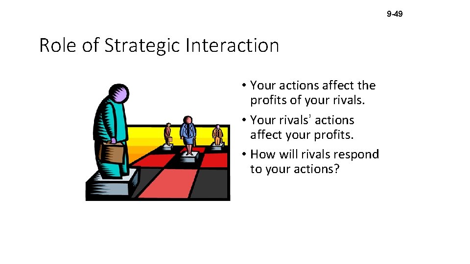
9 -49 Role of Strategic Interaction • Your actions affect the profits of your rivals. • Your rivals’ actions affect your profits. • How will rivals respond to your actions?

9 -50 An Example • You and another firm sell differentiated products. • How does the quantity demanded for your product change when you change your price?

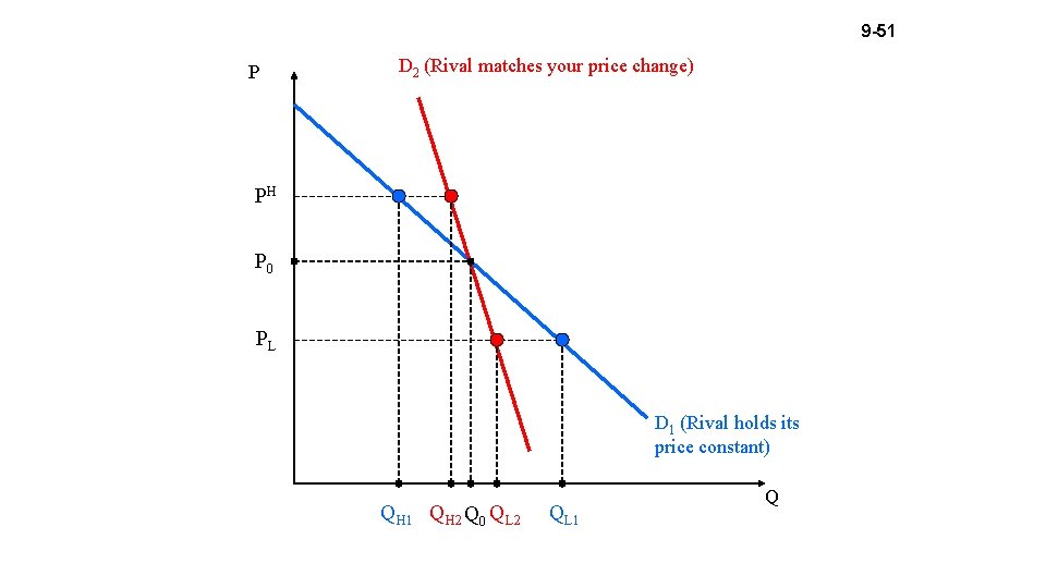
9 -51 P D 2 (Rival matches your price change) PH P 0 PL D 1 (Rival holds its price constant) QH 1 QH 2 Q 0 QL 2 QL 1 Q

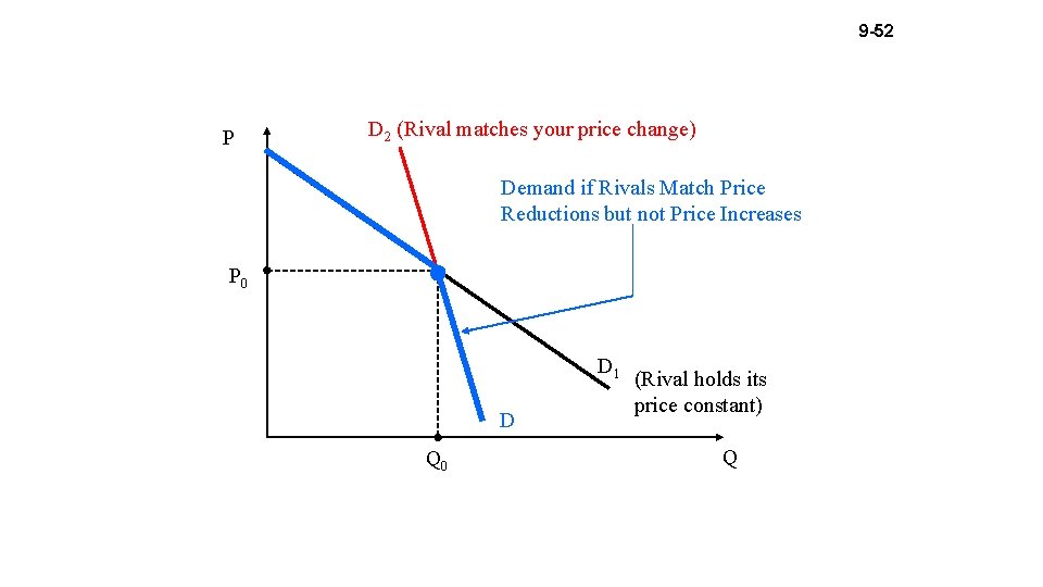
9 -52 P D 2 (Rival matches your price change) Demand if Rivals Match Price Reductions but not Price Increases P 0 D 1 D Q 0 (Rival holds its price constant) Q

9 -53 Key Insight • The effect of a price reduction on the quantity demanded of your product depends upon whether your rivals respond by cutting their prices too! • The effect of a price increase on the quantity demanded of your product depends upon whether your rivals respond by raising their prices too! • Strategic interdependence: You aren’t in complete control of your own destiny!

9 -54 Sweezy (Kinked-Demand) Model Environment Few firms in the market serving many consumers. Firms produce differentiated products. Barriers to entry. Each firm believes rivals will match (or follow) price reductions, but won’t match (or follow) price increases. • Key feature of Sweezy Model • • • Price-Rigidity.

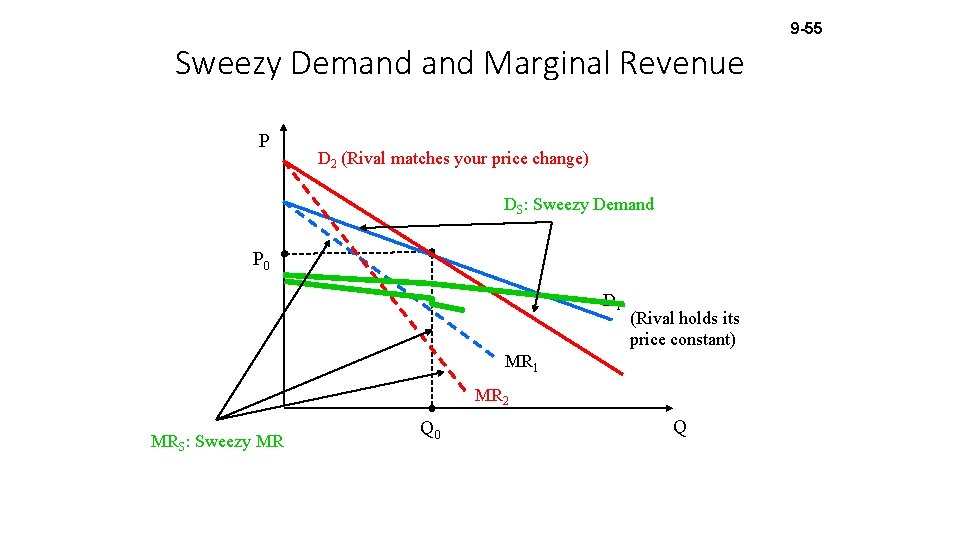
9 -55 Sweezy Demand Marginal Revenue P D 2 (Rival matches your price change) DS: Sweezy Demand P 0 D 1 (Rival holds its price constant) MR 1 MR 2 MRS: Sweezy MR Q 0 Q

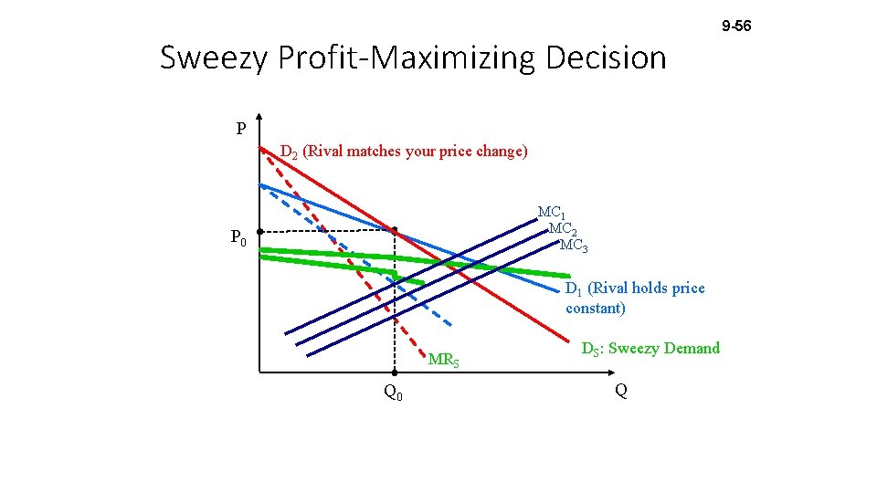
Sweezy Profit-Maximizing Decision P D 2 (Rival matches your price change) MC 1 MC 2 MC 3 P 0 D 1 (Rival holds price constant) MRS Q 0 DS: Sweezy Demand Q 9 -56

9 -57 Sweezy Oligopoly Summary • Firms believe rivals match price cuts, but not price increases. • Firms operating in a Sweezy oligopoly maximize profit by producing where MRS = MC. • The kinked-shaped marginal revenue curve implies that there exists a range over which changes in MC will not impact the profit-maximizing level of output. • Therefore, the firm may have no incentive to change price provided that marginal cost remains in a given range.

Cournot Model Environment • A few firms produce goods that are either perfect substitutes (homogeneous) or imperfect substitutes (differentiated). • Firms’ control variable is output in contrast to price. • Each firm believes their rivals will hold output constant if it changes its own output (The output of rivals is viewed as given or “fixed”). • Barriers to entry exist. 9 -58

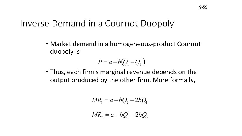
9 -59 Inverse Demand in a Cournot Duopoly • Market demand in a homogeneous-product Cournot duopoly is • Thus, each firm’s marginal revenue depends on the output produced by the other firm. More formally,

Best-Response Function 9 -60 • Since a firm’s marginal revenue in a homogeneous Cournot oligopoly depends on both its output and its rivals, each firm needs a way to “respond” to rival’s output decisions. • Firm 1’s best-response (or reaction) function is a schedule summarizing the amount of Q 1 firm 1 should produce in order to maximize its profits for each quantity of Q 2 produced by firm 2. • Since the products are substitutes, an increase in firm 2’s output leads to a decrease in the profit-maximizing amount of firm 1’s product.

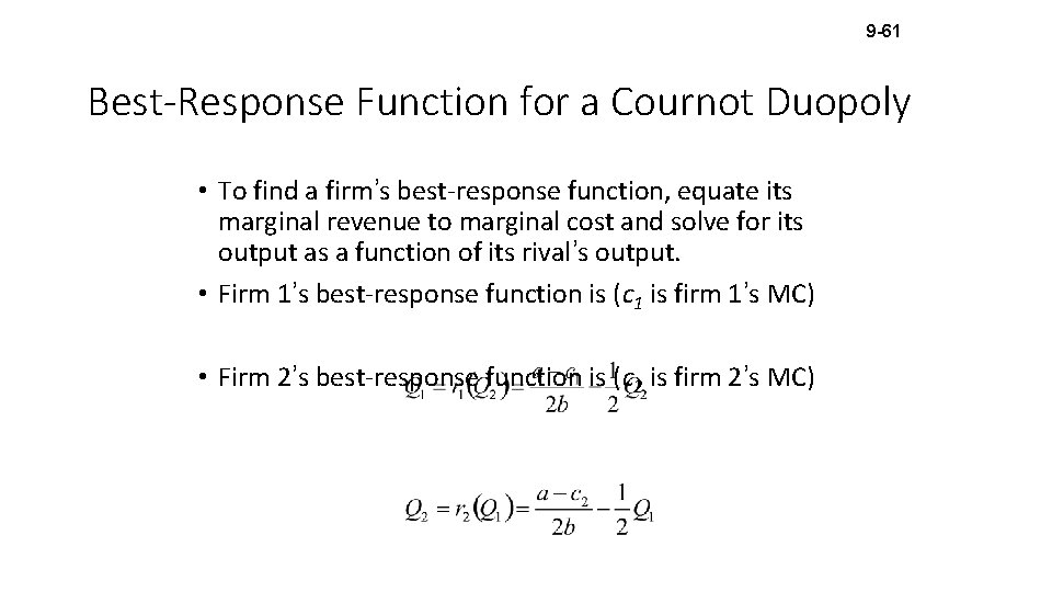
9 -61 Best-Response Function for a Cournot Duopoly • To find a firm’s best-response function, equate its marginal revenue to marginal cost and solve for its output as a function of its rival’s output. • Firm 1’s best-response function is (c 1 is firm 1’s MC) • Firm 2’s best-response function is (c 2 is firm 2’s MC)

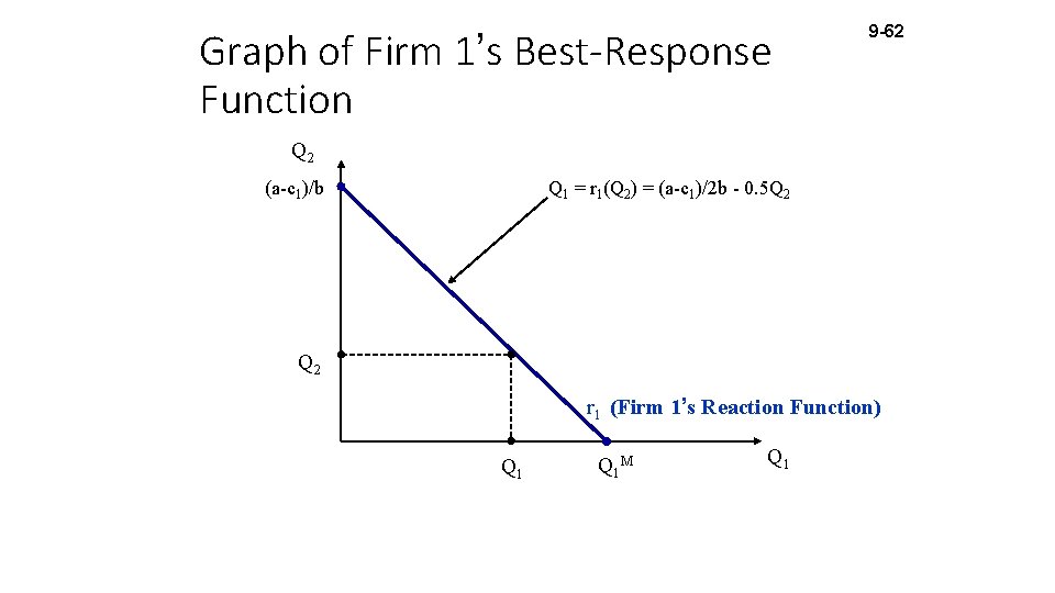
Graph of Firm 1’s Best-Response Function 9 -62 Q 2 (a-c 1)/b Q 1 = r 1(Q 2) = (a-c 1)/2 b - 0. 5 Q 2 r 1 (Firm 1’s Reaction Function) Q 1 M Q 1

9 -63 Cournot Equilibrium • Situation where each firm produces the output that maximizes its profits, given the output of rival firms. • No firm can gain by unilaterally changing its own output to improve its profit. • A point where the two firm’s best-response functions intersect.

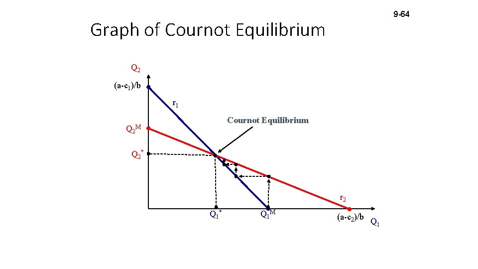
9 -64 Graph of Cournot Equilibrium Q 2 (a-c 1)/b r 1 Q 2 Cournot Equilibrium M Q 2 * r 2 Q 1 * Q 1 M (a-c 2)/b Q 1

Summary of Cournot Equilibrium • The output Q 1* maximizes firm 1’s profits, given that firm 2 produces Q 2*. • The output Q 2* maximizes firm 2’s profits, given that firm 1 produces Q 1*. • Neither firm has an incentive to change its output, given the output of the rival. • Beliefs are consistent: • In equilibrium, each firm “thinks” rivals will stick to their current output – and they do! 9 -65

9 -66 Stackelberg Model Environment • Few firms serving many consumers. • Firms produce differentiated or homogeneous products. • Barriers to entry. • Firm one is the leader. • The leader commits to an output before all other firms. • Remaining firms are followers. • They choose their outputs so as to maximize profits, given the leader’s output.

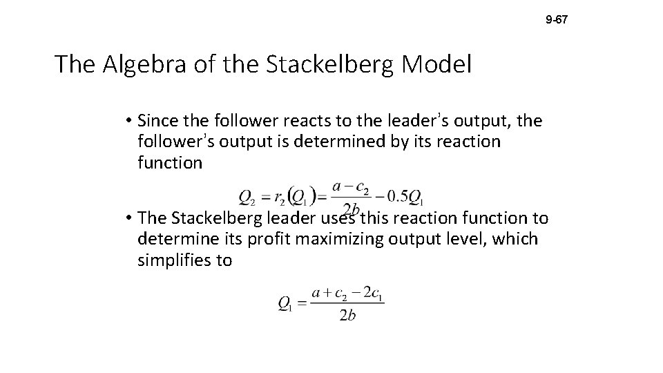
9 -67 The Algebra of the Stackelberg Model • Since the follower reacts to the leader’s output, the follower’s output is determined by its reaction function • The Stackelberg leader uses this reaction function to determine its profit maximizing output level, which simplifies to

Stackelberg Summary • Stackelberg model illustrates how commitment can enhance profits in strategic environments. • Leader produces more than the Cournot equilibrium output. • Larger market share, higher profits. • First-mover advantage. • Follower produces less than the Cournot equilibrium output. • Smaller market share, lower profits. 9 -68

9 -69 Bertrand Model Environment • Few firms that sell to many consumers. • Firms produce identical products at constant marginal cost. • Each firm independently sets its price in order to maximize profits (price is each firms’ control variable). • Barriers to entry exist. • Consumers enjoy • Perfect information. • Zero transaction costs.

Bertrand Equilibrium • Firms set P 1 = P 2 = MC! Why? • Suppose MC < P 1 < P 2. • Firm 1 earns (P 1 - MC) on each unit sold, while firm 2 earns nothing. • Firm 2 has an incentive to slightly undercut firm 1’s price to capture the entire market. • Firm 1 then has an incentive to undercut firm 2’s price. This undercutting continues. . . • Equilibrium: Each firm charges P 1 = P 2 = MC. 9 -70

9 -71 Conclusion • Different oligopoly scenarios give rise to different optimal strategies and different outcomes. • Your optimal price and output depends on … • Beliefs about the reactions of rivals. • Your choice variable (P or Q) and the nature of the product market (differentiated or homogeneous products). • Your ability to credibly commit prior to your rivals.