Management Strategy Evaluation and the Gulf of Alaska

Management Strategy Evaluation and the Gulf of Alaska walleye pollock fishery: including indicators of decadal change Teresa A’mar André Punt University of Washington Martin Dorn NOAA – NMFS, Alaska Fisheries Science Center 28 August 2007

Outline • Objectives • Management Strategy Evaluation • MSE and the Gulf of Alaska walleye pollock fishery • Regime shifts • Environmental variability • Next steps

Objectives • Examine the performance of the current management strategy under several hypotheses about decadal change in productivity • Evaluate alternative management strategies that are designed to be more responsive to decadal changes in productivity • Examine methods of incorporating indicators of environmental change into advice for fisheries management

Management Strategy Evaluation • Simulation testing of a feedback-control management strategy – accounting for process, measurement and model uncertainty – using performance measures based on identified management goals and objectives • This method is used in other countries, IWC

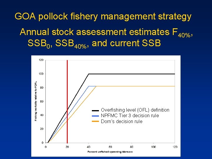
GOA pollock fishery management strategy Annual stock assessment estimates F 40%, SSB 0, SSB 40%, and current SSB Overfishing level (OFL) definition NPFMC Tier 3 decision rule Dorn’s decision rule

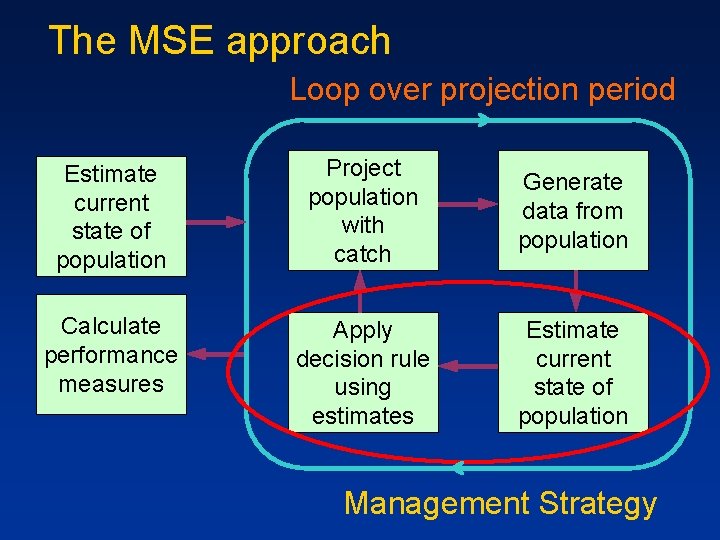
The MSE approach Loop over projection period Estimate current state of population Project population with catch Generate data from population Calculate performance measures Apply decision rule using estimates Estimate current state of population Management Strategy

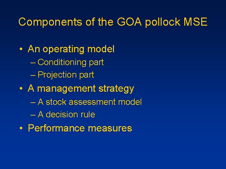
Components of the GOA pollock MSE • An operating model – Conditioning part – Projection part • A management strategy – A stock assessment model – A decision rule • Performance measures

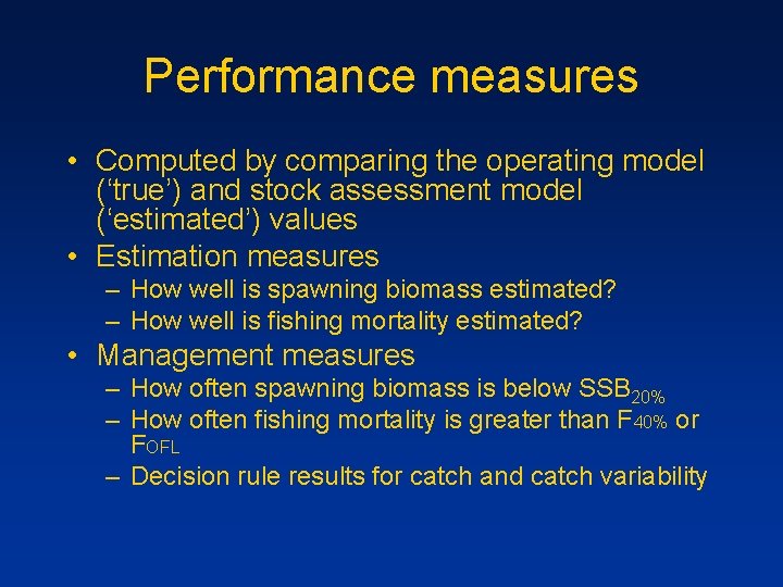
Performance measures • Computed by comparing the operating model (‘true’) and stock assessment model (‘estimated’) values • Estimation measures – How well is spawning biomass estimated? – How well is fishing mortality estimated? • Management measures – How often spawning biomass is below SSB 20% – How often fishing mortality is greater than F 40% or FOFL – Decision rule results for catch and catch variability

Simulations • The operating model estimates the state of the population in 2005 for simulations that start in 2006 • Bayesian analysis characterizes parameter uncertainty (a subset of 100 MCMC parameter vectors is used for the simulations) • Each simulated population is projected forward with uncorrelated process error and catches set by the management strategy • There is uncorrelated observation error in the data generated for the stock assessment

Some results

Simulation scenarios • Base scenario – 30 years, 2006 – 2035 – No environmental or ecosystem forcing • Regime shift – 50 years, 2006 – 2055 – Changes in average level of recruitment • Environmental variability – 45 years, 2006 – 2050 – Climate indices affect annual recruitment • Dorn’s decision rule is used in all scenarios

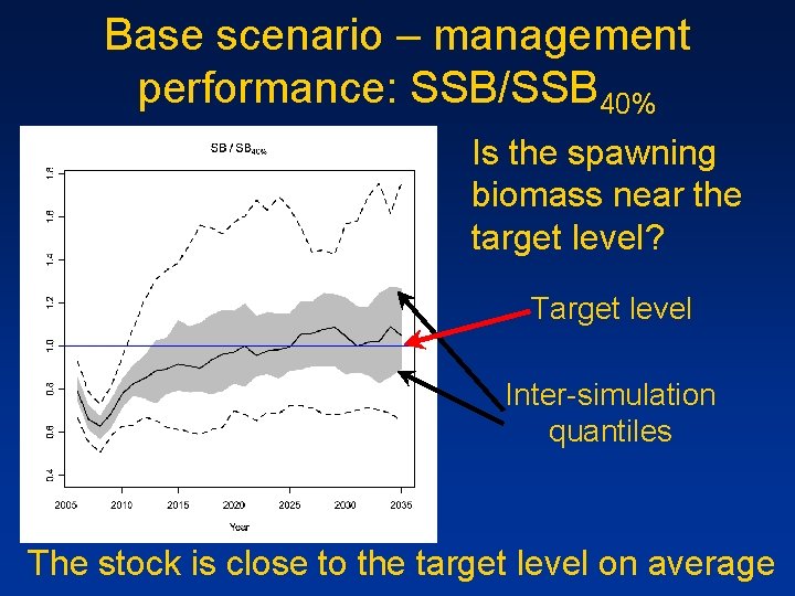
Base scenario – management performance: SSB/SSB 40% Is the spawning biomass near the target level? Target level Inter-simulation quantiles The stock is close to the target level on average

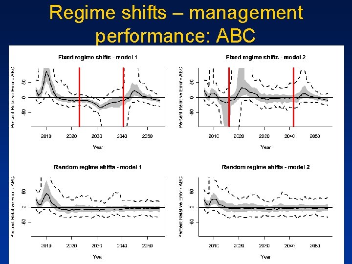
Base scenario – management performance: ABC Annual management decision based on assessment results and decision rule Errory = 100(Esty-Truey)/Truey

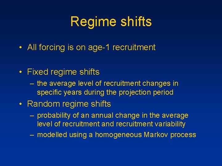
Regime shifts • All forcing is on age-1 recruitment • Fixed regime shifts – the average level of recruitment changes in specific years during the projection period • Random regime shifts – probability of an annual change in the average level of recruitment and recruitment variability – modelled using a homogeneous Markov process

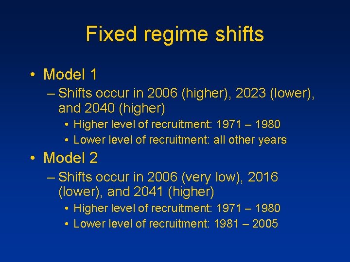
Fixed regime shifts • Model 1 – Shifts occur in 2006 (higher), 2023 (lower), and 2040 (higher) • Higher level of recruitment: 1971 – 1980 • Lower level of recruitment: all other years • Model 2 – Shifts occur in 2006 (very low), 2016 (lower), and 2041 (higher) • Higher level of recruitment: 1971 – 1980 • Lower level of recruitment: 1981 – 2005

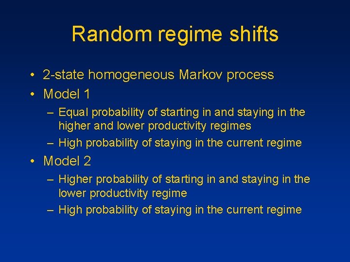
Random regime shifts • 2 -state homogeneous Markov process • Model 1 – Equal probability of starting in and staying in the higher and lower productivity regimes – High probability of staying in the current regime • Model 2 – Higher probability of starting in and staying in the lower productivity regime – High probability of staying in the current regime

Regime shifts – management performance: SSB/SSB 40%

Regime shifts – management performance: ABC

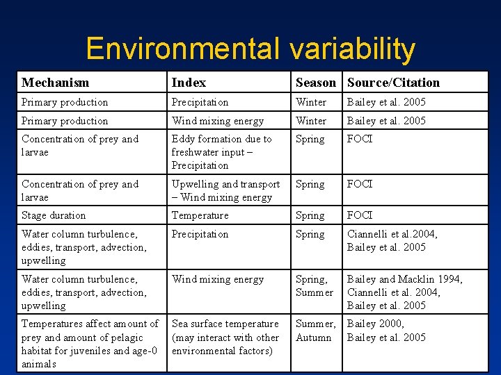
Environmental variability Mechanism Index Season Source/Citation Primary production Precipitation Winter Bailey et al. 2005 Primary production Wind mixing energy Winter Bailey et al. 2005 Concentration of prey and larvae Eddy formation due to freshwater input – Precipitation Spring FOCI Concentration of prey and larvae Upwelling and transport – Wind mixing energy Spring FOCI Stage duration Temperature Spring FOCI Water column turbulence, eddies, transport, advection, upwelling Precipitation Spring Ciannelli et al. 2004, Bailey et al. 2005 Water column turbulence, eddies, transport, advection, upwelling Wind mixing energy Spring, Summer Bailey and Macklin 1994, Ciannelli et al. 2004, Bailey et al. 2005 Temperatures affect amount of prey and amount of pelagic habitat for juveniles and age-0 animals Sea surface temperature (may interact with other environmental factors) Summer, Autumn Bailey 2000, Bailey et al. 2005

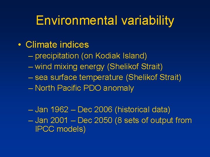
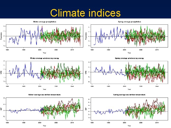
Environmental variability • Climate indices – precipitation (on Kodiak Island) – wind mixing energy (Shelikof Strait) – sea surface temperature (Shelikof Strait) – North Pacific PDO anomaly – Jan 1962 – Dec 2006 (historical data) – Jan 2001 – Dec 2050 (8 sets of output from IPCC models)

Climate indices

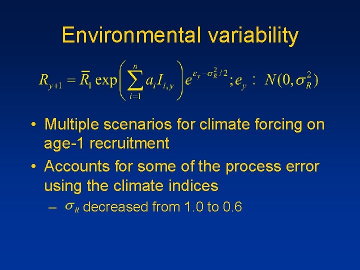
Environmental variability • Multiple scenarios for climate forcing on age-1 recruitment • Accounts for some of the process error using the climate indices – decreased from 1. 0 to 0. 6

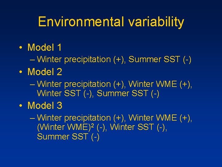
Environmental variability • Model 1 – Winter precipitation (+), Summer SST (-) • Model 2 – Winter precipitation (+), Winter WME (+), Winter SST (-), Summer SST (-) • Model 3 – Winter precipitation (+), Winter WME (+), (Winter WME)2 (-), Winter SST (-), Summer SST (-)

Environmental variability – management performance: SSB/SSB 40%

Environmental variability – management performance: ABC

Next steps

Alternative management strategies • Use 25 -year sliding window for average recruitment used in calculating SSB 40% • Develop software to detect regime shifts using estimated age-2 recruitment – Rodionov and Overland (2005) – Find change points using sequential t-test analysis • Use results of regime shift analysis to influence how the biological reference points are calculated changes in ABC

Acknowledgements • André Punt, Martin Dorn, Ray Hilborn, and Dan Huppert • Funding through NOAA FATE • Anne Hollowed, Nick Bond, Bern Megrey • NOAA Personnel at AFSC • The Punt Lab at UW