Management oriented process based models The 3 PG

Management oriented process based models The 3 PG model as an example Analysis of the original 3 PG

Summary r Main diferences to empirical models r Overview of 3 PG (brief) b Growth module b Calculus module b Management module r The 3 PGpjs 2. 7. xls implementation r Exercises

Main differences to empirical models

3 PG is r. A tree growth model based on Physiological Principles that Predict Growth r. Bridges the gap between mensuration-based growth and yield models and process-based, carbon balance models r. Provides fully dynamic predictions of biomass pools and soil water use r. Includes process-based and empirical relationships (some consider them as an “hybrid” model) r. Is based on a monthly time step

r. Advantages bapplicable under changing conditions bcan be adapted for a range of species bparameterised using stand-level data bprovides explanation, aids understanding r. Disadvantages bnot as widely understood as empirical growth models bnot necessarily as accurate when applied to the current situation bcan require data not readily available b. In the original 3 PG, less detailed output bnaïve treatment of soil nutrition ballocation based largely on size bpoor predictor of canopy development and of mortality

Input data r Climate data b monthly mean temperature, radiation, rainfall, VPD b observed or long-term average data of the same variables r Site and soil descriptors b latitude b soil texture and maximum soil water capacity b fertility rating (0 -1) r Also need stand initialisation data b foliage, stem+bark+branches and root biomass b stocking

Outputs - monthly (original 3 PG) r Biomass pools (wood+bark+branches, leaves and roots) r Stocking r Available soil water r NPP r Evapotranspiration r Average dbh r Underbark volume r Stand basal area

Overview of 3 PG

Main components of 3 PG r Growth module: b Production of biomass – environmental modification of light use efficiency; constant ratio of NPP to GPP b Biomass allocation – affected by growing conditions +tree size b Stem mortality – probability of death; self-thinning b Soil water balance – single soil layer model; evapotranspiration determined from Penman. Monteith equation r Calculus module b Stand properties – from biomass pools and assumptions about specific leaf area, branch+bark fraction, and wood density

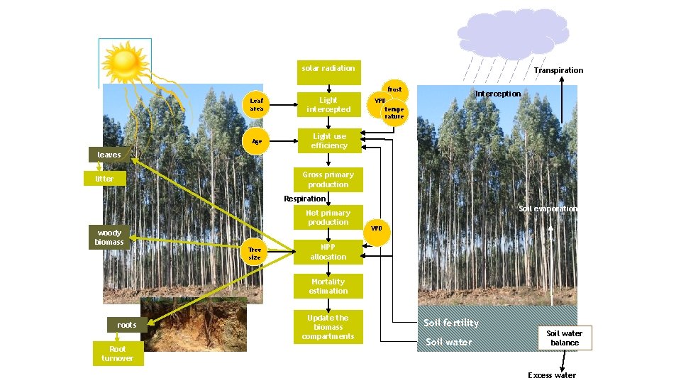
solar radiation Transpiration frost Leaf area Light intercepted Age Light use efficiency Interception VPD tempe rature leaves Gross primary production litter Respiration Net primary production woody biomass Tree size Soil evaporation VPD NPP allocation Mortality estimation roots Root turnover Update the biomass compartments Soil fertility Soil water balance Excess water

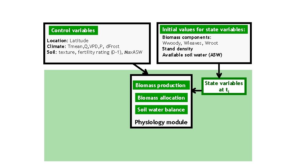
Initial values for state variables: Control variables Location: Latitude Climate: Tmean, Q, VPD, P, d. Frost Soil: texture, fertility rating (0 -1), Max. ASW Biomass components: Wwoody, Wleaves, Wroot Stand density Available soil water (ASW) Biomass production Biomass allocation Soil water balance Physiology module State variables at ti

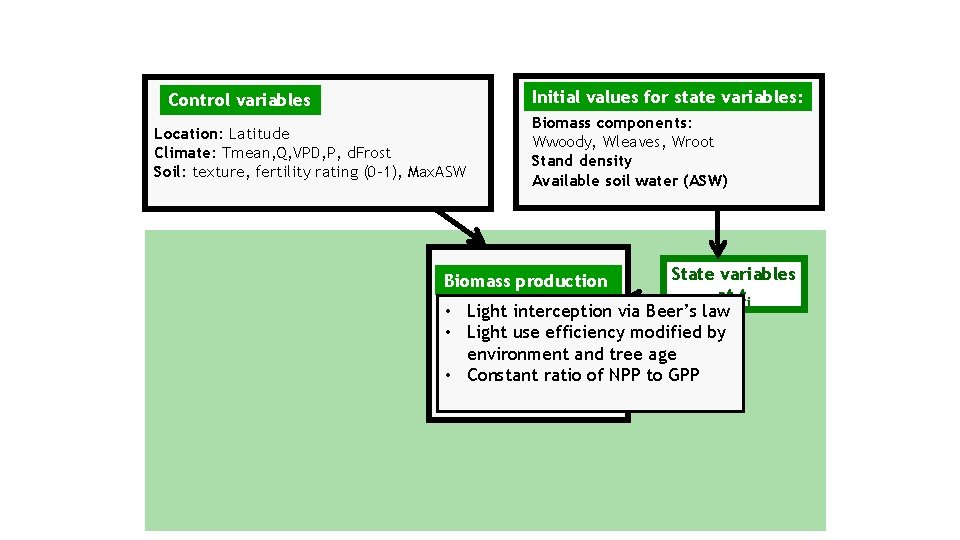
Initial values for state variables: Control variables Location: Latitude Climate: Tmean, Q, VPD, P, d. Frost Soil: texture, fertility rating (0 -1), Max. ASW Biomass components: Wwoody, Wleaves, Wroot Stand density Available soil water (ASW) State variables at ti • Light interception via Beer’s law Biomass allocation • Light use efficiency modified by environment and tree age Soil water balance • Constant ratio of NPP to GPP Biomass production Physiology module

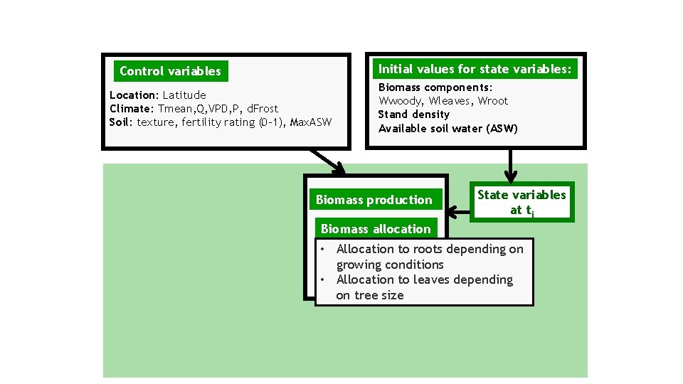
Initial values for state variables: Control variables Location: Latitude Climate: Tmean, Q, VPD, P, d. Frost Soil: texture, fertility rating (0 -1), Max. ASW Biomass components: Wwoody, Wleaves, Wroot Stand density Available soil water (ASW) Biomass production State variables at ti Biomass allocation • Allocation to roots depending on Soil water balance growing conditions • Allocation to leaves depending Physiology module on tree size

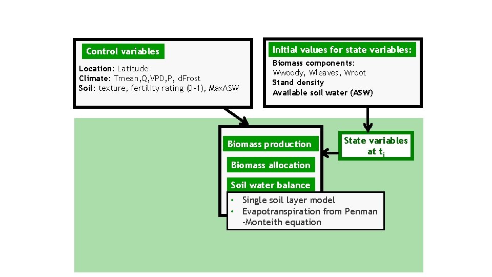
Initial values for state variables: Control variables Location: Latitude Climate: Tmean, Q, VPD, P, d. Frost Soil: texture, fertility rating (0 -1), Max. ASW Biomass components: Wwoody, Wleaves, Wroot Stand density Available soil water (ASW) Biomass production State variables at ti Biomass allocation Soil water balance • Single soil layer model Physiology module from Penman • Evapotranspiration -Monteith equation

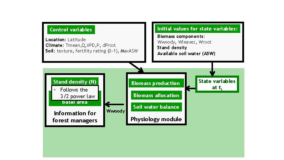
Initial values for state variables: Control variables Location: Latitude Climate: Tmean, Q, VPD, P, d. Frost Soil: texture, fertility rating (0 -1), Max. ASW Stand density (N) • Follows the Volume under law bark 3/2 power Basal area Information forest managers Biomass components: Wwoody, Wleaves, Wroot Stand density Available soil water (ASW) Biomass production Biomass allocation Wwoody Soil water balance Physiology module State variables at ti

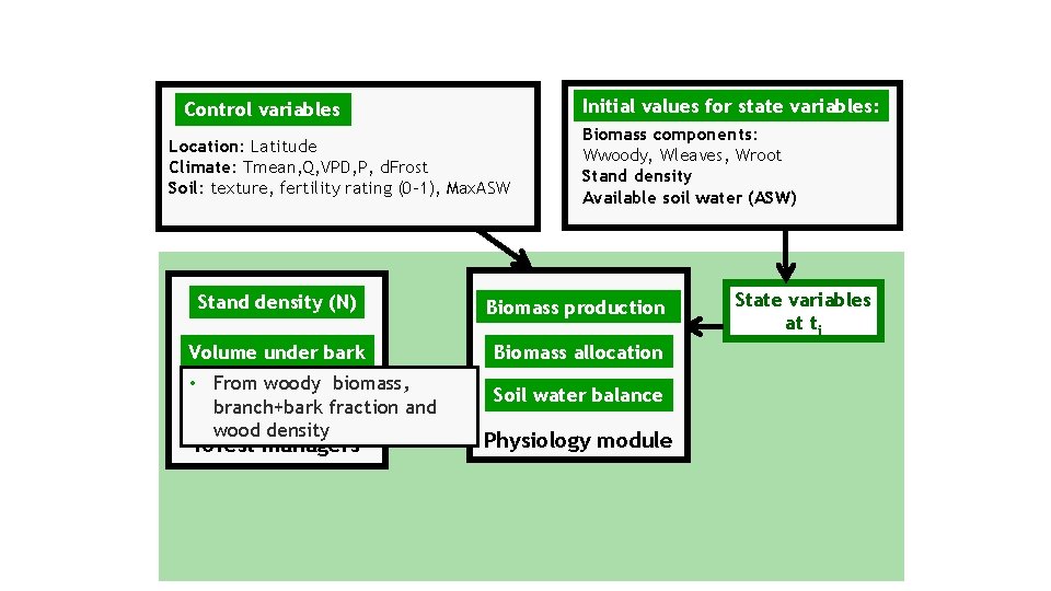
Initial values for state variables: Control variables Location: Latitude Climate: Tmean, Q, VPD, P, d. Frost Soil: texture, fertility rating (0 -1), Max. ASW Stand density (N) Volume under bark Basal area biomass, • From woody branch+bark fraction. Wwoody and Information for wood density forest managers Biomass components: Wwoody, Wleaves, Wroot Stand density Available soil water (ASW) Biomass production Biomass allocation Soil water balance Physiology module State variables at ti

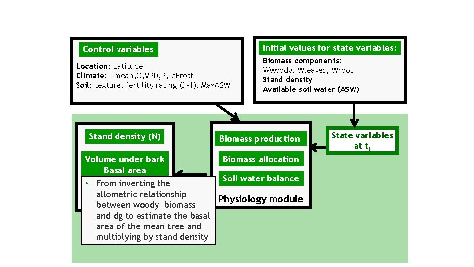
Initial values for state variables: Control variables Location: Latitude Climate: Tmean, Q, VPD, P, d. Frost Soil: texture, fertility rating (0 -1), Max. ASW Biomass components: Wwoody, Wleaves, Wroot Stand density Available soil water (ASW) Stand density (N) Biomass production Volume under bark Basal area Biomass allocation Soil water balance • From inverting the Wwoody Information for allometric relationship Physiology module forest managers between woody biomass and dg to estimate the basal area of the mean tree and multiplying by stand density State variables at ti

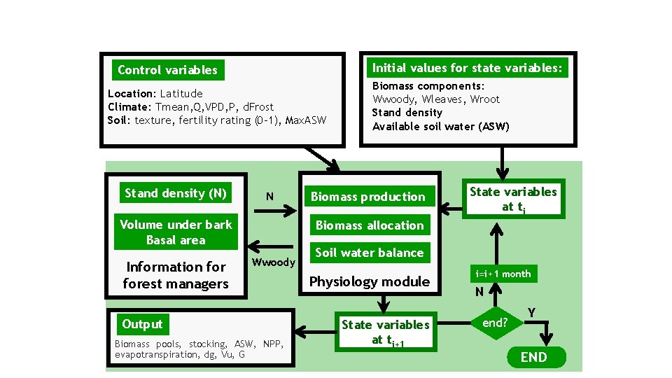
Initial values for state variables: Control variables Location: Latitude Climate: Tmean, Q, VPD, P, d. Frost Soil: texture, fertility rating (0 -1), Max. ASW Stand density (N) N Volume under bark Basal area Information forest managers Biomass components: Wwoody, Wleaves, Wroot Stand density Available soil water (ASW) Biomass production State variables at ti Biomass allocation Wwoody Output Biomass pools, stocking, ASW, NPP, evapotranspiration, dg, Vu, G Soil water balance Physiology module State variables at ti+1 i=i+1 month N end? Y END

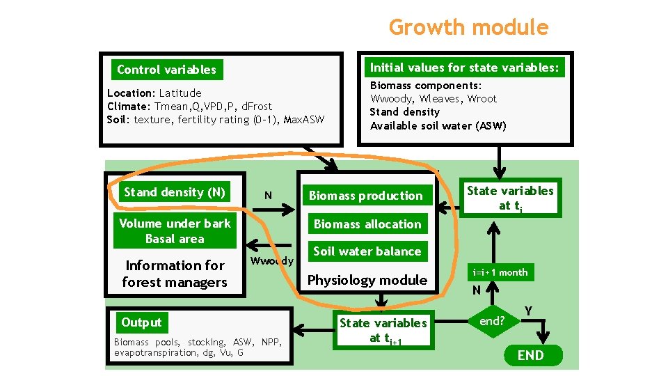
Growth module Initial values for state variables: Control variables Location: Latitude Climate: Tmean, Q, VPD, P, d. Frost Soil: texture, fertility rating (0 -1), Max. ASW Stand density (N) N Volume under bark Basal area Information forest managers Biomass components: Wwoody, Wleaves, Wroot Stand density Available soil water (ASW) Biomass production State variables at ti Biomass allocation Wwoody Output Biomass pools, stocking, ASW, NPP, evapotranspiration, dg, Vu, G Soil water balance Physiology module State variables at ti+1 i=i+1 month N end? Y END

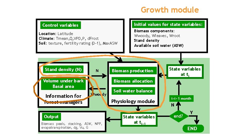
Growth module Initial values for state variables: Control variables Location: Latitude Climate: Tmean, Q, VPD, P, d. Frost Soil: texture, fertility rating (0 -1), Max. ASW Stand density (N) N Volume under bark Basal area Information forest managers Biomass components: Wwoody, Wleaves, Wroot Stand density Available soil water (ASW) Biomass production State variables at ti Biomass allocation Wwoody Output Biomass pools, stocking, ASW, NPP, evapotranspiration, dg, Vu, G Soil water balance Physiology module State variables at ti+1 i=i+1 month N end? Y END

Overview of 3 PG Biomass production

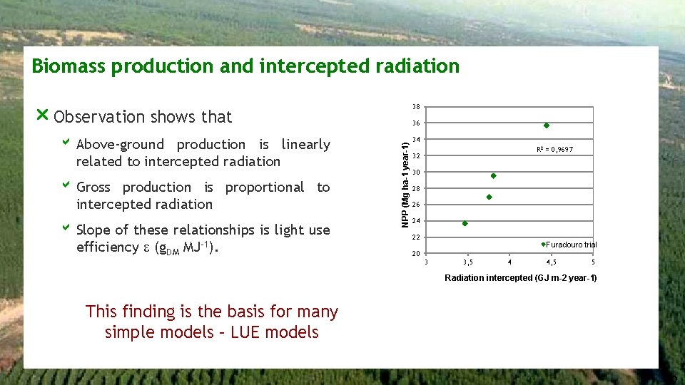
Biomass production and intercepted radiation 38 r Observation shows that b Gross production is proportional to intercepted radiation b Slope of these relationships is light use efficiency (g. DM MJ-1). NPP (Mg ha-1 year-1) b Above-ground production is linearly related to intercepted radiation 36 34 R 2 = 0, 9697 32 30 28 26 24 22 Furadouro trial 20 3 3, 5 4 4, 5 5 Radiation intercepted (GJ m-2 year-1) This finding is the basis for many simple models – LUE models

Light use efficiency r Is affected by climatic factors (e. g. temperature) and site factors (e. g. soil-water status) r Varies seasonally, but annual values more stable r Gross production is affected by modifiers – functions that vary between 0 and 1 – related with climatic and site factors (multiplicative or according to the law of minimum)

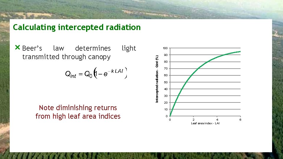
Calculating intercepted radiation Note diminishing returns from high leaf area indices light 100 Intercepted radiation - Qint (%) r Beer’s law determines transmitted through canopy 90 80 70 60 50 40 30 20 10 0 0 2 4 Leaf area index - LAI 6

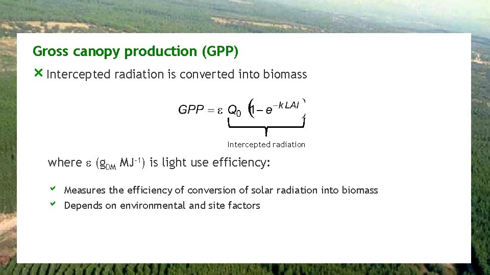
Gross canopy production (GPP) r Intercepted radiation is converted into biomass Intercepted radiation where (g. DM MJ-1) is light use efficiency: b Measures the efficiency of conversion of solar radiation into biomass b Depends on environmental and site factors

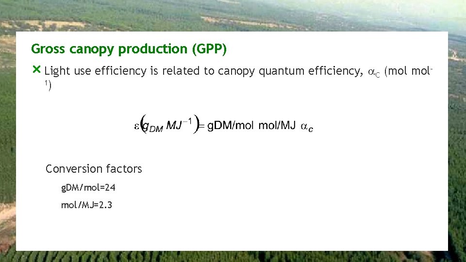
Gross canopy production (GPP) r Light use efficiency is related to canopy quantum efficiency, C (mol 1) Conversion factors g. DM/mol=24 mol/MJ=2. 3

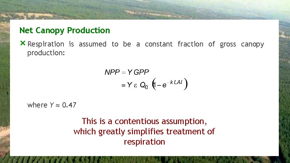
Net Canopy Production r Respiration is assumed to be a constant fraction of gross canopy production: where Y 0. 47 This is a contentious assumption, which greatly simplifies treatment of respiration

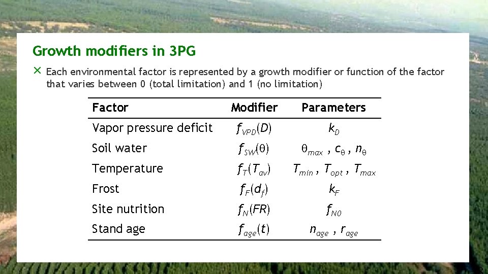
Growth modifiers in 3 PG r Each environmental factor is represented by a growth modifier or function of the factor that varies between 0 (total limitation) and 1 (no limitation) Factor Modifier Parameters Vapor pressure deficit f. VPD(D) k. D Soil water f. SW( ) max , c , n Temperature f. T(Tav) Tmin , Topt , Tmax Frost f. F(df) k. F Site nutrition f. N(FR) f. N 0 Stand age fage(t) nage , rage

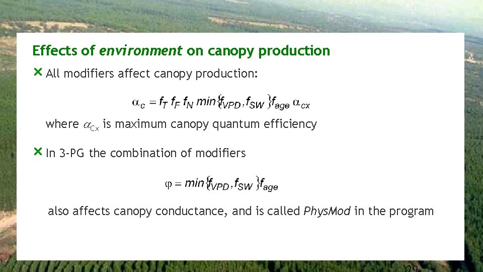
Effects of environment on canopy production r All modifiers affect canopy production: where Cx is maximum canopy quantum efficiency r In 3 -PG the combination of modifiers also affects canopy conductance, and is called Phys. Mod in the program

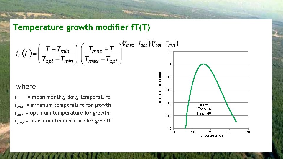
Temperature growth modifier f. T(T) 1, 2 where T = mean monthly daily temperature Tmin = minimum temperature for growth Topt = optimum temperature for growth Tmax = maximum temperature for growth Temperature modifier 1 0, 8 0, 6 0, 4 Tmin= 6 Topt= 16 Tmax= 40 0, 2 0 0 10 20 Temperature (ºC) 30 40

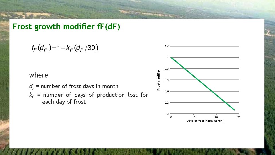
Frost growth modifier f. F(d. F) 1, 2 where d. F = number of frost days in month k. F = number of days of production lost for each day of frost Frost modifier 1 0, 8 0, 6 0, 4 0, 2 0 0 10 20 Days of frost in the month) 30

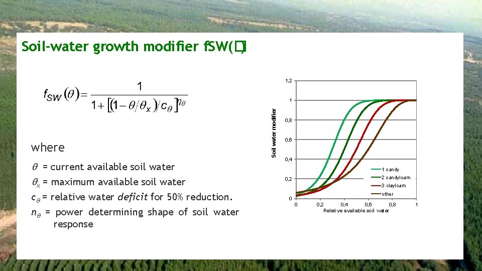
Soil-water growth modifier f. SW(�) 1, 2 where = current available soil water x = maximum available soil water c = relative water deficit for 50% reduction. n = power determining shape of soil water response Soil water modifier 1 0, 8 0, 6 0, 4 1 sandy 2 sandyloam 0, 2 3 clayloam other 0 0 0, 2 0, 4 0, 6 0, 8 Relative available soil water 1

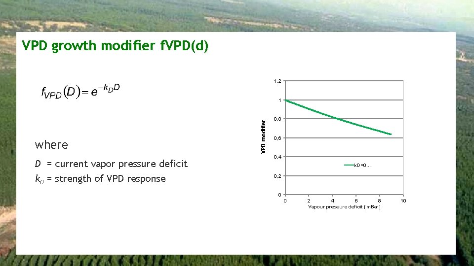
VPD growth modifier f. VPD(d) 1, 2 where D = current vapor pressure deficit k. D = strength of VPD response VPD modifier 1 0, 8 0, 6 0, 4 k. D=0. . 0, 2 0 0 2 4 6 8 Vapour pressure deficit (m. Bar) 10

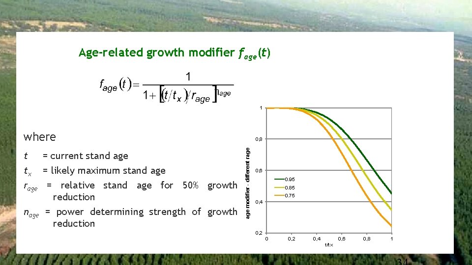
Age-related growth modifier fage(t) 1 where age modifier - different rage t = current stand age tx = likely maximum stand age rage = relative stand age for 50% growth reduction nage = power determining strength of growth reduction 0, 8 0, 6 0. 95 0. 85 0. 75 0, 4 0, 2 0, 4 0, 6 t/tx 0, 8 1

Overview of 3 PG Biomass partitioning

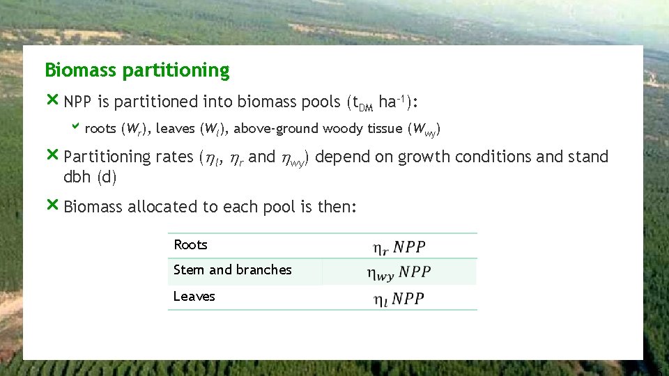
Biomass partitioning r NPP is partitioned into biomass pools (t. DM ha-1): b roots (Wr), leaves (Wl), above-ground woody tissue (Wwy) r Partitioning rates ( l, r and wy) depend on growth conditions and stand dbh (d) r Biomass allocated to each pool is then: Roots Stem and branches Leaves

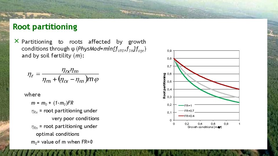
Root partitioning r Partitioning to roots affected by growth conditions through j (Phys. Mod=min{f. VPD, f. SW}fage) and by soil fertility (m): 0, 9 0, 8 where m = m 0 + (1 -m 0)FR Rx = root partitioning under very poor conditions Rn = root partitioning under optimal conditions m 0= value of m when FR=0 Root partitioning 0, 7 0, 6 0, 5 0, 4 0, 3 0, 2 FR=1 FR=0. 7 0, 1 FR=0. 4 0 0 0, 2 0, 4 0, 6 0, 8 Growth conditions (m ) 1

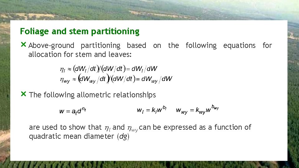
Foliage and stem partitioning r Above-ground partitioning based on the following equations for allocation for stem and leaves: r The following allometric relationships are used to show that l and wy can be expressed as a function of quadratic mean diameter (dg)

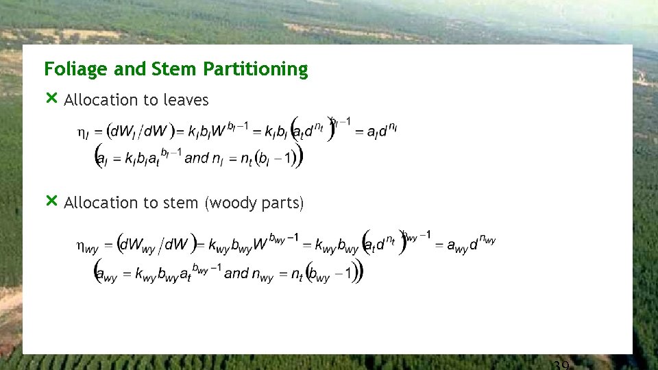
Foliage and Stem Partitioning r Allocation to leaves r Allocation to stem (woody parts)

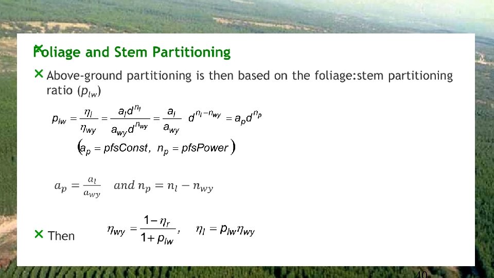
r

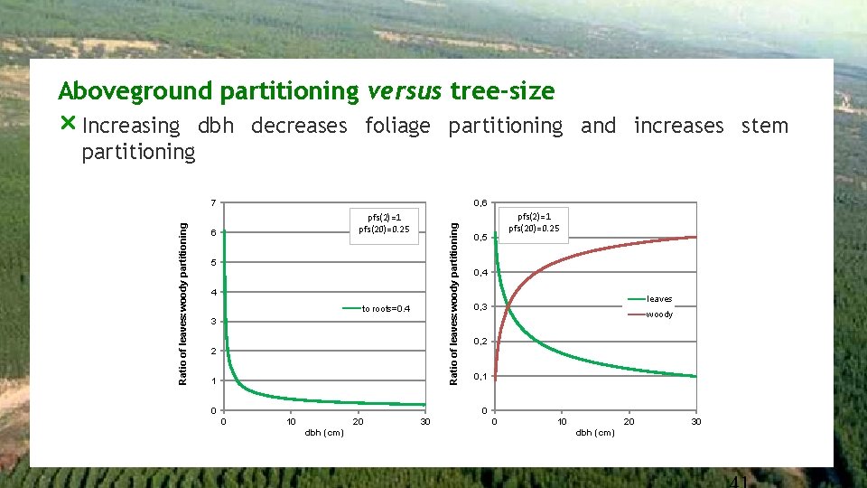
Aboveground partitioning versus tree-size r Increasing dbh decreases foliage partitioning and increases stem partitioning 0, 6 pfs(2)=1 pfs(20)=0. 25 6 Ratio of leaves: woody partitioning 7 5 4 to roots=0. 4 3 2 1 0 pfs(2)=1 pfs(20)=0. 25 0, 4 leaves 0, 3 woody 0, 2 0, 1 0 0 10 20 dbh (cm) 30

Overview of 3 PG Monthly biomass update

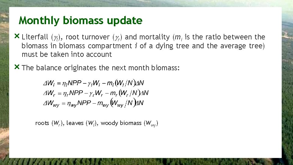
Monthly biomass update r Literfall (gl), root turnover (gr) and mortality (mi is the ratio between the biomass in biomass compartment i of a dying tree and the average tree) must be taken into account r The balance originates the next month biomass: roots (Wr), leaves (Wl), woody biomass (Wwy)

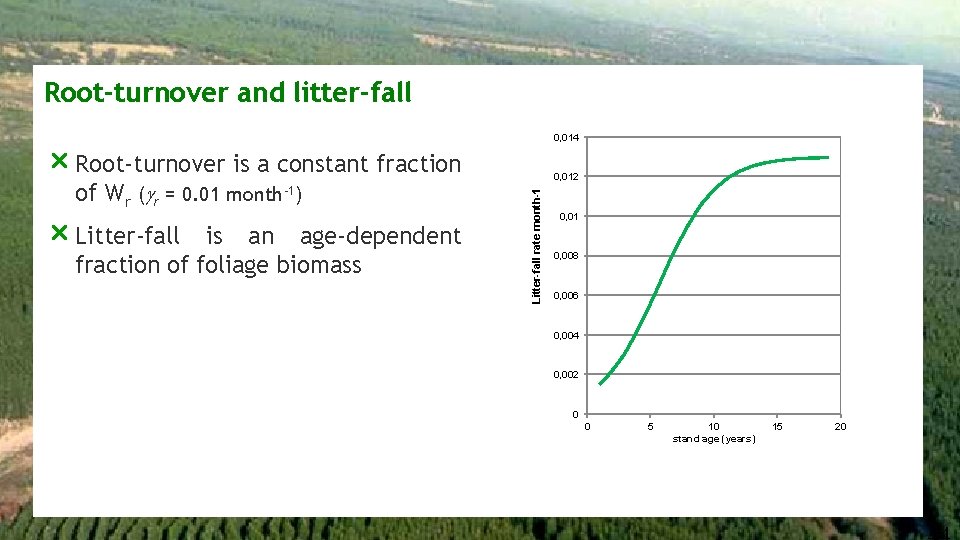
Root-turnover and litter-fall 0, 014 r Litter-fall is an age-dependent fraction of foliage biomass 0, 012 Litter-fall rate month-1 r Root-turnover is a constant fraction of Wr (gr = 0. 01 month-1) 0, 01 0, 008 0, 006 0, 004 0, 002 0 0 5 10 stand age (years) 15 20

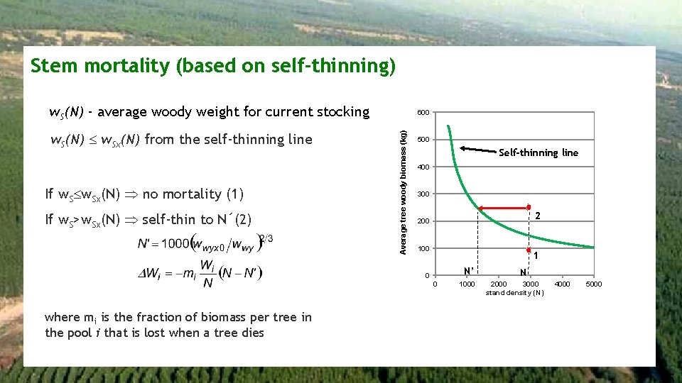
Stem mortality (based on self-thinning) w. S(N) - average woody weight for current stocking If w. Sx(N) no mortality (1) If w. S>w. Sx(N) self-thin to N´(2) Average tree woody biomass (kg) w. S(N) w. Sx(N) from the self-thinning line 600 500 Self-thinning line 400 300 2 200 1 N’ 0 0 where mi is the fraction of biomass per tree in the pool i that is lost when a tree dies 1000 N 2000 3000 stand density (N) 4000 5000

Overview of 3 PG Soil water balance

Soil water balance r Soil water balance based on single soil layer r Uses monthly time steps Inputs: b rainfall and irrigation Losses are: b interception = fixed % of rainfall b evapotranspiration – Penman-Monteith equation b excess over field capacity lost as run off

Evapotranspiration r Evapotranspiration is calculated using the Penman-Monteith equation b Directly affected by VPD and radiation r Canopy conductance: b determined by LAI b affected by growth conditions – VPD, soil water and age r Boundary layer conductance: b is assumed constant (0. 2 m s-1)

Overview of 3 PG Management module

Fertilization and irrigation r Fertilization can be considered by changing the fertility rating (FR) parameter r Irrigation can be considered in several ways (in 3 PGpjs 27. xls): : 1. By adding it to the precipitation days 2. By indicating a value of minimum available soil water different from zero – it starts irrigation as soon as this threshold is attained 3. By providing a list of ages and Ml ha-1 year-1 – it will changes the amount of irrigation at every year indicated in the list

Thinning r Thinning is simulated by indicating: 1. The year of thinning 2. Thinning intensity – periodicity by selecting the years for thinning, it is possible to simulate several thinnings along the rotation 3. Thinning severity – number of trees that are thinned 4. Thinning type – ratio of biomass of leaves, woody and roots of an average thinned tree and an average tree of the stand

Defoliation r Defoliation can be considered by indicating 1. The year 2. The percentage of leaves that remain r There is a recent tool, developed for Portugal, that simulates the impact of defoliation using the 3 PG model

Overview of 3 PG Calculus module (original 3 PG)

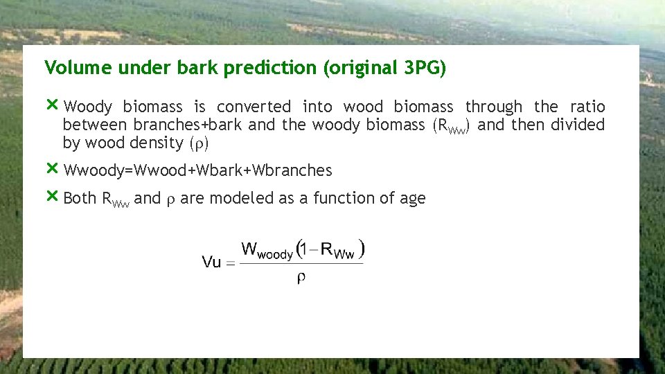
Volume under bark prediction (original 3 PG) r Woody biomass is converted into wood biomass through the ratio between branches+bark and the woody biomass (RWw) and then divided by wood density ( ) r Wwoody=Wwood+Wbark+Wbranches r Both RWw and are modeled as a function of age

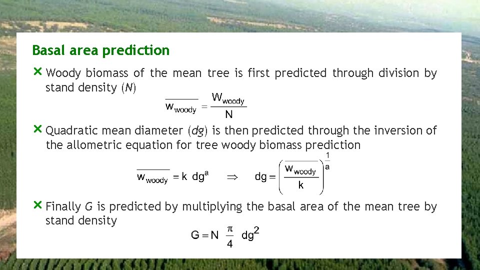
Basal area prediction r Woody biomass of the mean tree is first predicted through division by stand density (N) r Quadratic mean diameter (dg) is then predicted through the inversion of the allometric equation for tree woody biomass prediction r Finally G is predicted by multiplying the basal area of the mean tree by stand density

The 3 PGpjs_2. 7 EXCEL file

r 3 PG is implemented in Visual Basic for applications as an Add-ins for EXCEL, available in the site 3 pg. forestry. ubc. ca/software b To install 3 PGpjs proceed as follows: a) Download the 3 PGpjs 27. zip and extract all files and folders in 3 PGpjs 27. zip to a folder of your choice b) Open 3 PGPJS 27. xls and save it as 3 PGpjs 27. xla (Excel Add-in) c) To load the 3 PGpjs add-in go to Excel’s TOOLS|ADD-INS menu, select GO and then place a tick against the ‘ 3 PGpjs 27’ add-in name. If you do not see this listed, use the BROWSE button to locate it. d) You can also unload the add-in by repeating this process and removing the tick mark e) The EXCEL file 3 PGpjs 27. Data is prepared to run 3 PG in 32 -bits computers

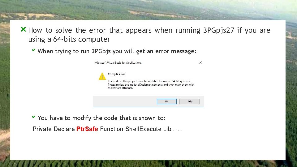
r How to solve the error that appears when running 3 PGpjs 27 if you are using a 64 -bits computer b When trying to run 3 PGpjs you will get an error message: b You have to modify the code that is shown to: Private Declare Ptr. Safe Function Shell. Execute Lib …. .

The end!!!